George E. P. Box famously described the problem of model development in statistics and related fields by noting, all models are wrong, but some are useful(1976). That is, all models are necessarily simplifications of a much more complex reality and statistics is by no means an algorithmic truth generating process because no model can ever be true in the pure sense of the word. Yet, this at times underappreciated reality does not render all models useless but rather implies the goal of those who practice statistics in its various forms is to develop and identify models that are useful in a never ending quest to be less wrong. In this post I introduce an approach to this task that has been the subject of my own dissertation work on the use of Bayesian Model Averaging (BMA) to account for uncertainty in model specification when estimating average marginal effects in non-linear regression models.
I outline here what I term a Bayesian Model Averaged Marginal Effect (BMAME) in the context of logistic regression models in political science and illustrate how to obtain BMAMEs in a straightforward manner using the marginaleffects R package (Arel-Bundock 2022), which thanks to Vincent Arel-Bundock’s assistance supports model averaged or stacked average marginal effects for any model fit with the Stan interface brms(Bürkner 2017, 2018). I also provide a more general demonstration in Stan that makes the method easily applicable in Python and high dimensional settings. Although I focus here on models that include only population-level effects, recent feature additions to marginaleffects now make it possible to obtain BMAMEs from more complex hierarchical models and I will cover such applications in a subsequent post.
In minor contrast to the past advice of Montgomery and Nyhan (2010) who suggest “BMA is best used as a subsequent robustness check to show that our inferences are not overly sensitive to plausible variations in model specification” (266), I argue here model averaging can and should be used as far more than a robustness check if for no other reason than a model-wise mixture distribution for the paramter of interest is almost certainly more informative than a point estimate from a single model specification. Indeed, BMA provides one of the few natural and intuitive ways of resolving some of the issues outlined in the preceding paragraph, particularly as it pertains to the evaluation of non-nested theoretical models, while also exhibiting a lower false positive rate than alternative approaches (Plümper and Traunmüller 2018). This section provides a brief explanation of BMA and its connection to model averaged marginal effects before proceeding to a discussion of how the procedure is implemented.
Bayesian Model Comparison and Model Averaging
Consider a simple case in which we have a set of \(\mathcal{M}\) models, each of which characterizes a possible representation of some unknown data generation process. Although it remains common practice in applied political science to select a single model based on a largely arbitrary fit statistic (i.e., AIC, \(\chi^{2}\), or whatever people are getting a p-value from this week), such an approach is problematic since it ignores the uncertainty inherent in the process of model specification. Rather than selecting a single model and consequently placing an implicit zero prior on every other possible model specification you could have reasonably considered but did not, Bayesian Model Averaging and its analogues provide a means of averaging across several possible, potentially non-nested, model specifications and accounting for the uncertainty associated with doing so.
Imagine we wish to adjudicate between two competing theoretical models in the set of candidate models \(\mathcal{M}\). The posterior odds of model \(i\) relative to an alternative \(k\) can be expressed as
where \(\pi(\mathcal{M})\) is the prior probability of model \(i\) over model \(k\) and \(p(y \,|\, \mathcal{M})\) is the marginal likelihood of the observed data under each of the candidate models such that
Given our prior assumptions about how likely the observed data are to have arisen from each model in the set \(\mathcal{M}\), the result of equation 1 is the posterior odds of model \(i\) compared to model \(k\) and thus captures the relative probability that model \(\mathcal{M_{i}}\) represents the true data generation process compared to the plausible alternative \(\mathcal{M_{k}}\). We can easily extend this example to the setting in which \(\mathcal{M_{k}}\) is a set of plausible competing models of size \(k > 2\), in which case the posterior model probability of the \(i^{th}\) model relative to each of the alternatives \(k\) is
Applying equation 3 to each model in the set under consideration yields a vector of relative posterior model probabilities of length \(m\) which may be used as either posterior probability weights as in the case of Bayesian Model Averaging or for the estimation of posterior inclusion probabilities.
In the context of model averaging, we can take draws from the posterior predictive distribution of each model containing a given parameter of interest proportional to its posterior probability weight obtained from equation 3. This yields a model-wise mixture representing a weighted average of the posterior predictive distribution for some parameter such as a regression coefficient for a linear model or as I outline below, an average marginal effect or probability contrast for models that employ a non-linear link function.
Bayesian Model Averaged Marginal Effects
Average marginal effects are ubquitous in the social sciences though, as Andrew Heiss nicely illustrates, the term average marginal effect is often used ambiguously and in the context of more complex models, the terms marginal and conditional tend to be a source of additional confusion. In the case of a simple population-level linear model with a Gaussian likelihood and identity link function, the model averaged marginal effect is equivalent to the posterior distribution of the model averaged coefficient \(\beta\) which can be expressed as
where \(\Pr(\mathcal{M}_{i} ~ | ~ y)\) represent the posterior model probability and \(\mathbb{E}(\beta ~|~ \mathcal{M}_{i}, ~ y)\) is the expected value of some parameter \(\beta\) conditional on the observed data and some model specification for each model \(i\) in the set of models under consideration \(m\)(Montgomery and Nyhan 2010).
For probability models such as logit, and other commonly used formulations for modeling discrete responses, this simple closed form solution does not exist nor is there any meaningful way to interpret the coefficients of these models as efffect size estimates–a reality that unfortunately remains quite widely misunderstood (Daniel, Zhang, and Farewell 2020; Mood 2009). As a general principle, any model more complex than a simple linear regression can only be meaningfully interpreted in terms of the predictions it generates(Long and Mustillo 2018), which in the case of logistic regression simply means applying the inverse logistic function to obtain predicted probabilities which we can then use to estimate contrasts or average marginal effects (Norton, Dowd, and Maciejewski 2019). Letting \(\mathrm{Y}\) represent a binary outcome, \(\mathrm{X}\) a continuous exposure or treatment of interest, and \(\mathrm{Z}\) a matrix of measured confounders, we can express the average marginal effect as
which provided a sufficiently small value of \(h\), yields a reasonable approximation of the partial derivative and provides a posterior distribution for the average effect of an instantaneous change in \(\mathrm{X}\) on the probability scale similar to what one obtains in linear regression.
Similarly, for a binary treatment of interest we apply the Bayesian g-formula to obtain the average marginal effect of \(\mathrm{X}\) on the probability of \(\mathrm{Y}\) as shown in equation 6.
Equations 5 and 6 make clear we are averaging over the confounder distribution \(\mathrm{Z}\) rather than holding it constant at some fixed value (Keil et al. 2017; Oganisian and Roy 2020). This point is an important one because in binary outcome models such as logit and probit, holding \(\mathrm{Z}\) constant at some fixed value such as the mean corresponds to an entirely different estimand(Hanmer and Kalkan 2012). The AME is a population-averaged quantity, corresponding to the population average treatment effect and these two quantities can produce very different results under fairly general conditions because they do not answer the same question.
From here it is straightforward to obtain a model averaged marginal effect estimate for a discrete outcome model such as logit. Given marginal predictions for each model \(k\) in the set \(m\), we can apply equation 7 to obtain the posterior distribution of average marginal effects for each model.
This yields a model-wise mixture distribution representing the weighted average of the marginal effects estimates and has broad applicability to scenarios common in the social sciences, industry, and any other setting where a need arises to account for uncertainty in model specification.
Limitations and Caveats
While traditional marginal likelihood-based Bayesian model averaging is a powerful and principled technique for dealing with uncertainty in the process of model specification and selection, it is not without limitations and caveats of its own, some of which bear emphasizing before proceeding further.
Marginal Likelihood and Computational Uncertainty
First, for all but the simplest of models attempting to derive the integral in equation 2 analytically proves to be computationally intractable and we must instead rely on algorithmic approximations such as bridge sampling (Gelman and Meng 1998; Gronau et al. 2017; Wang, Jones, and Meng 2020). While the bridge sampling approximation tends to perform well compared to common alternatives, estimates of the marginal likelihood \(p(y \,|\, \mathcal{M})\) may be highly variable upon repeated runs of the algorithm (Schad et al. 2022). This problem tends to arise in more complex hierarchical models with multiple varying effects and, perhaps unsurprisingly, suggests that by relying on approximations we introduce an additional source of computational uncertainty that may need to be accounted for.
For the purposes of BMAMEs, I have elsewhere proposed addressing this additional source of uncertainty and incorporating it into the estimates by executing the bridge sampling algorithm \(S\) times for each model to obtain a distribution of possible values for the approximate log marginal likelihood. Given a vector of estimates for \(p(y ~|~ \mathcal{M})\) of length \(s\) for each model \(k \in \{1,2,\dots, m\}\), we can apply equation 3 to obtain an \(s \times m\) matrix of posterior model probabilities. It is then straightforward to extend equation 7 to average over the distribution of posterior probability weights rather than relying on single estimate or point estimate as shown in equation 8 below.2
Whether this approach is necessary depends largely on how variable the algorithm is on repeated runs and it may simply be adequate to instead take the median or mean of the marginal likelihood estimates for each model. Although it is beyond the scope of this post, one could also use exhaustive leave-future-out cross-validation which is equivalent to the marginal likelihood given a logarithmic scoring rule (Bürkner, Gabry, and Vehtari 2020; Fong and Holmes 2020), though this approach tends to be extremely expensive in terms of computation.
Bayes Factors and Prior Sensitivity
The second caveat with respect to obtaining BMAMEs stems from a common criticism of Bayes Factors. Although as the amount of available data \(n \longrightarrow \infty\), the likelihood will tend to dominate the prior in Bayesian estimation, this is not necessarily the case in terms of inference. Indeed, from equations 2 and 3 one can quite clearly see the the posterior probability \(\Pr(\mathcal{M} ~| ~y)\) depends on the prior probability of the parameters, \(\pi(\theta \,|\, \mathcal{M})\) in equation 2, and the respective prior probability \(\pi(\mathcal{M})\) of each model in the set under consideration. Since our substantive conclusions may be sensitive to either of these prior specifications, these assumptions should be checked to verify the results do not vary wildly under reasonable alternatives.
Perhaps more importantly, due to their dependence on Bayes Factors, posterior probability weights require at least moderatlely informative priors on each and every parameter in a model and it is by this point common knowledge that specifying a flat or “uninformative” prior such as \(\beta \sim \mathrm{Uniform(-\infty, \infty)}\) or even an excessively vague one tends to bias Bayes Factors–and by extension values that depend on them–violently in favor of the null model.3 This is a feature of applied Bayesian inference rather than a bug and if you make stupid assumptions, you will arrive at stupid conclusions. The solution to this problem is to think carefully about the universe of possible effect sizes you might observe for a given parameter, assign reasonable priors that constrain the parameter space, and verify the results are robust to alternative distributional assumptions.
Likeihoods and Priors
The degree to which a prior can be considered informative is heavily dependent on the likelihood and can often only be understood in that context (Gelman, Simpson, and Betancourt 2017).
Stacking, and the Open-\(\mathcal{M}\) Problem
Finally, traditional BMA is flawed in the sense that its validity rests upon the closed \(\mathcal{M}\) assumption implicit in equation 3. In the open \(\mathcal{M}\) setting where the true model is not among those in the set of candidate models under consideration, as will generally be the case in any real world application, estimated effects based on posterior probability weights are likely to be biased (Hollenbach and Montgomery 2020; Yao et al. 2018). This problem arises from the fact that marginal-likelihood based posterior probability weights for each model \(m \in \mathcal{M}\) correspond to the probability a given model captures the true data generation process and in most settings this is unlikely to ever be the case since, by definition, all models are wrong.
In the open \(\mathcal{M}\) setting, traditional BMA will still assign each model some probability but since by definition \(\sum_{i=1}^{m}\Pr(\mathcal{M}_{i} ~|~ y) = 1\), these weights no longer have a valid interpretation in terms of the posterior probability a given model is true. Although this does not render marginal likelihood based model averaging useless and it may often make more sense to think about model specification and selection as a probabilistic process aimed at identifying the most likely model conditional on the set of models under consideration (Hinne et al. 2020), it is advisable to assess whether our substantive conclusions are sensitive to potential violations of the closed \(\mathcal{M}\) assumption. This once again underscores the fact that statistics is not a mechanistic truth generating process and there is no magic. It also underscores the need to think in more local terms–rather than asking is this model true we generally want to know the probability \(\mathrm{X}\) belongs to the true data generation process.4
An alternative but still properly Bayesian approach aimed at addressing these potential flaws in traditional BMA is cross-validation based stacking (Yao et al. 2018). In contrast to traditional BMA, stacking and pseudo-BMA weights are constructed based on the relative expectation of the posterior predictive density (Hollenbach and Montgomery 2020; Yao et al. 2018). These approaches to estimating model weights do not rely upon the closed \(\mathcal{M}\) assumption, and thus provide a way of either avoiding it altogether or relaxing it as a robustness check on the posterior probability weights, albeit while answering a fundamentally different question more appropriate for an open \(\mathcal{M}\) world. Since the overall approach to calculating model averaged AMEs does not change and we are merely substituting the posterior probability weights in equation 7 with stacking or pseudo-BMA weights, I direct readers to Yao et al. (2018) for a formal discussion of these approaches.
Female Combatants and Post-Conflict Rebel Parties
To illustrate the utility of BMAMEs in political science, I draw on an example adapted from the second chapter of my dissertation in which I examine how the active participation of women in rebel groups during wartime shapes the political calculus of former combatant groups at war’s end. In short, I expect rebel groups where women participate in combat roles during wartime to be more likely to form political parties and participate in post-conflict elections.
Data
To identify the universe of post-conflict successor parties to former combatant groups I rely on the Civil War Successor Party (CWSP) dataset which includes all civil wars in the UCDP Armed Conflicts Dataset (UCDP) that terminated between 1970 and 2015 (Daly 2020). Since the primary distinction between political parties and other civil society organizations such as interest groups lies in the latter’s participation in elections and fielding candidates for political office and a party that does not compete in elections is no party at all, I operationalize our dependent variable, Rebel to Party Transition, as a binary event which takes a value of 1 if a rebel group both forms a political party and directly participates in a country’s first post-conflict elections and 0 otherwise. The resulting sample consists of 112 observations for 108 unique rebel groups across 56 countries, approximately 66% of which formed parties and participated in their country’s first post-conflict election.
Following Wood and Thomas (2017), I define female combatants as members of a rebel group who are “armed and participate in organized combat activities on behalf of a rebel organization” (38). I code instances of female participation in rebel groups by mapping version 1.4 of the Women in Armed Rebellion Data (WARD) to the CWSP and construct two versions of the main predictor of interest based on the best estimate for the presence of female combatants in a given rebel group, one of which includes cases in which women served only as suicide bombers while the other codes these groups as not having any women in combat positions. Each of these variables takes a value of 1 if women participated in combat in a given rebel group and 0 otherwise. Among the rebel groups in our analysis, female combatants have been active in some capacity in 52.67% of those who were involved in civil wars that have terminated since 1970 and 50.89% featured women in non-suicide bombing roles.
I also adjust for several additional factors that may otherwise confound the estimate of the effect of female participation in combat on rebel successor party transitions. First, insurgent groups that attempt to perform functions typically characteristic of the state during wartime may be more likely to transition to political parties following the end of a conflict since, in doing so, they both develop organizational capacity and if successful, demonstrate that they are capable of governing to their future base of support. Moreover, as rebel groups build organizational capacity and accumulate institutional knowledge, their ability to sustain a successful insurgency and recruit combatants grows as well. To adjust for rebel organizational capacity I specify a Bayesian multidimensional item response model to construct a latent scale capturing the degree to which rebel groups engaged in functions of the state during wartime based on twenty-six items from Quasi-State Institutions dataset (Albert 2022).
Second, I adjust for baseline characteristics of each rebel group that previous research suggests influences both where women rebel and post-conflict party transitions. Drawing on data from Braithwaite and Cunningham (2019), I construct a series of dichotomous indicator variables for whether a rebel group is affiliated with an existing political party (Manning and Smith 2016), nationalist and left-wing or communist ideological origins (Wood and Thomas 2017), and whether a group has ties to a specific ethnic community since this may provide advantages in terms of mobilizing combatants and voters along specific cleavages. I also construct two additional indictators to capture whether the United Nations intervened in the conflict and whether a given rebel group was located in Africa.
While it is, of course, impossible in the context of an observational setting such as this one to isolate every possible source of confounding, nor is it generally advisable to attempt to do so, I focus on these baseline covariates since existing research provides a strong theoretical basis to suspect they impact the relationship of interest.5 For the purposes of this illustration, I assume this set of covariates is sufficient to satisfy strong ignorability but such an assumption is likely unreasonable and the particular analysis here may ultimately best be taken as descriptive in nature.
Code
# Load the required librariespacman::p_load("tidyverse", "arrow","data.table","brms", "furrr", "cmdstanr","patchwork","ggdist","marginaleffects", install =FALSE)# Read in the pre-processed datamodel_df<-read_parquet("data/model_data.gz.parquet")
Model and Priors
To estimate the effect of women’s participation in combat on post-conflict rebel party transitions for this example, I specify a simple logit model as shown in equation 9. The bernoulli probability \(\mu\) of a rebel group transitioning to a political party at war’s end is modeled as a function of the population-level intercept \(\alpha\) and a vector of coefficients \(\beta_{k}\) corresponding to the matrix of inputs \(X_{n}\).
Since we model \(\mu\) via a logit link function, our priors on the intercept \(\alpha\) and coefficients \(\beta_{k}\) should correspond to the expected change in the log odds of the response for each predictor. Some may find the process of prior elicitation in logistic regression models difficult since reasoning on the logit scale may seem unintuitive. As figure 1 illustrates, the the log odds of the response for models with that employ a logit link function is effectively bounded between approximately \(-6\) and \(6\). Values in excess of \(|5|\) generally should not occur unless your data exhibits near complete or quasi-complete separation.
Code
## Simulate logit probabilitieslogit_scale<-tibble( x =seq(-6.5, 6.5, 0.0001), y =brms::inv_logit_scaled(x))## Plot the logit scaleggplot(logit_scale, aes(x =x, y =y))+## Add a line geomgeom_line(size =3, color ="firebrick")+## Add labelslabs(x ="Log Odds", y ="Probability")+## Adjust the x axis scale breaksscale_x_continuous(breaks =seq(-6, 6, 1))+## Adjust the y axis scale breaksscale_y_continuous(breaks =seq(0, 1, 0.1))
Figure 1: Scale of the Logit Link
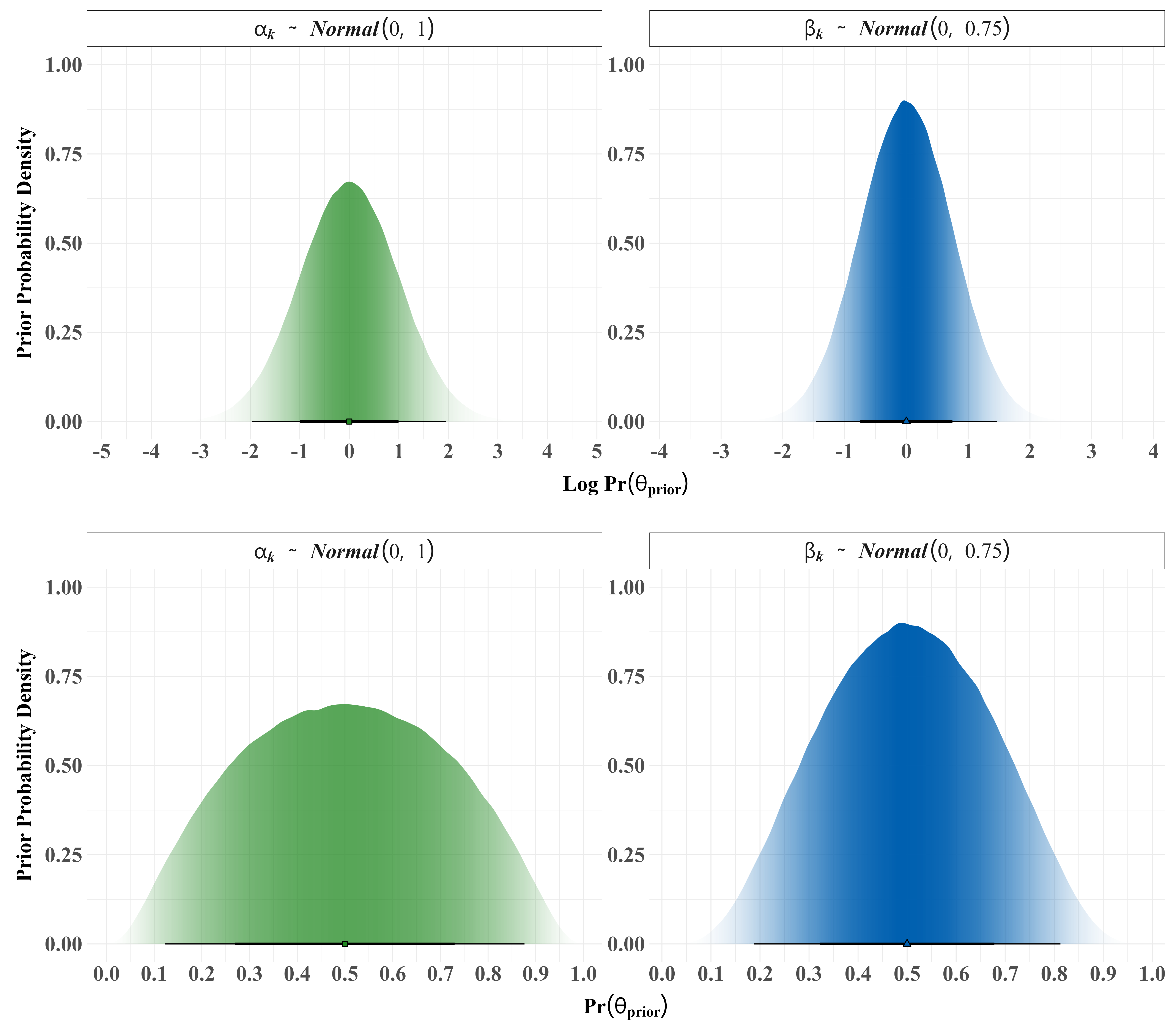
Framed in terms of effect sizes, a change of \(\pm 3\) in the log odds of the response relative to the baseline spans half the logit scale in either direction. In the social sciences where data is largely random noise and effect sizes are typically small to moderate at best and while the road to hell is paved with rules of thumb, we can generally assume a priori that 1) any true effect of a given parameter \(\beta\) in the population is likely modest in magnitude and 2) values closer zero are more likely than those further away. From these relatively straightforward assumptions, we can arrive at a prior for the coefficients that follows a normal distribution with mean 0 and scale \(0.75\) as shown in equation 9. In practical terms, this assumes the universe possible effect sizes for each predictor is normally distributed in the range of approximately \(-1.5\) and \(1.5\) on the logit scale.
For the population-level intercept \(\alpha\) I assign a slightly more diffuse normal prior mean 0 and scale 1 or \(\alpha \sim \text{Normal}(0,~1)\) which reflects a slightly greater degree of uncertainty about the baseline probability but is still moderately informative and constrains the bulk of the prior density in the range of realistic values. It is important to note here that as shown in Stan model below, we are specifying a prior on the intercept for the centered inputs rather than on the original scale. To more explicitly communicate our prior assumptions, we can use the tools for visualizing uncertainty provided in the ggdist package as shown in figure 2 below (Kay 2022).
Code
# Simulate the prior probabilitieslogit_priors<-tibble( alpha_prior =rnorm(10e5, 0, 1), beta_prior =rnorm(10e5, 0, 0.75))%>%## Pivot the simulated data to long formpivot_longer(everything())# Set parameter names for the facets----logit_prior_labels<-as_labeller( x =c("beta_prior"="bolditalic(beta[k] * phantom(.) * phantom() %~% phantom() * phantom(.) * Normal(0*list(,) * phantom(.) * 0.75))","alpha_prior"="bolditalic(alpha[k] * phantom(.) * phantom() %~% phantom() * phantom(.) * Normal(0*list(,) * phantom(.) * 1))"), default =label_parsed)# Plot the prior distributionslogit_prior_plots<-logit_priors%>%# Initiate the ggplot objectggplot(aes(x =value, fill =name, shape =name))+# Facet by the prior distributionsfacet_wrap(~name, scales ="free", labeller =logit_prior_labels)+# Add a half eye geom for the prior distributionsstat_halfeye(aes(slab_alpha =stat(pdf)), .width =c(.68, .95), fill_type ="gradient", show.legend =FALSE)+# Manually set the fill colorsscale_fill_manual(values =c("#208820", "#0060B0"))+# Manually set the shapesscale_shape_manual(values =c(22, 24))+# Adjust the breaks on the y axisscale_x_continuous(breaks =scales::pretty_breaks(n =8))+# Add labels to the plotlabs( y ="Prior Probability Density", x =latex2exp::TeX(r'(Log $\Pr(\theta_{prior})$)', bold =T))# Plot back transformed probabilitiesprob_trans_plots<-logit_priors%>%# Initiate the ggplot objectggplot(aes(fill =name, shape =name))+# Facet by the prior distributionsfacet_wrap(~name, scales ="free", labeller =logit_prior_labels)+# Add a half eye geom for the prior distributionsstat_halfeye(aes(x =plogis(value), slab_alpha =stat(pdf)), .width =c(.68, .95), fill_type ="gradient", show.legend =FALSE)+# Manually set the fill colorsscale_fill_manual(values =c("#208820", "#0060B0"))+# Manually set the shapesscale_shape_manual(values =c(22, 24))+# Add labels to the plotlabs( y ="Prior Probability Density", title ="", x =latex2exp::TeX(r'($\Pr(\theta_{prior})$)', bold =TRUE))+# Adjust the breaks on the x axisscale_x_continuous(breaks =scales::pretty_breaks(n =8))## Print the combined plotlogit_prior_plots/prob_trans_plots
Figure 2: Priors for the Logit Model Parameters
Since the model here is computationally quite efficient–on average, each model takes approximately 2.5 seconds to converge with 30,000 post-warmup draws–and in the interest of completeness, I search the full parameter space which consists of \(2^{k}\) possible model specifications. Although it is possible to do this in this context, researchers will often instead need to place constrain the number of possible model configurations, generally by specifying an implicit prior model probability of 1 for certain parameters (Hinne et al. 2020; Montgomery and Nyhan 2010). Although brms provides an easy to use R interface to Stan that makes fitting a wide variety of Bayesian regression models easier than ever before and requires no direct knowledge of Stan, it is limited for my purposes here by the fact that it requires recompiling the underlying Stan model for each fit. This process ends up being extremely inefficient for a large number of model configurations since each model takes three times as long to compile as it does to fit.
To circumvent this issue, I implement the model directly in Stan in a way designed to be directly compatible with brms. For models containing the parameter of interest, the model implments the bayesian g-formula to estimate the average marginal effect of women’s participation in combat on the probability of a rebel-to-party transition during the estimation process in the generated quanitites block. As I previously demonstrated in this post, it is then possible to compile the Stan model once and use the same program for each dataset using {cmdstanr} directly. Further computational gains can be obtained by using the furrr package to fit multiple models in parallel and I specify a series of functions to streamline this process as shown below.
// Bayesian Logit Model with Optional Bootstrapped AMEs via the Bayesian g-formuladata {int<lower=1> N; // N Observationsarray[N] int Y; // Response Variableint<lower=1> K; // Number of Population-Level Effectsmatrix[N, K] X; // Population-level Design Matrixint prior_only; // Should the likelihood be ignored?int treat_pos; // Data for the bootstrapped AMEs}transformed data {int Kc = K - 1;matrix[N, Kc] Xc; // centered version of X without an interceptvector[Kc] means_X; // column means of X before centeringfor (i in2 : K) { means_X[i - 1] = mean(X[ : , i]); Xc[ : , i - 1] = X[ : , i] - means_X[i - 1]; }// Bootstrap Probabilitiesvector[N] boot_probs = rep_vector(1.0/N, N);// Matrices for the bootstrapped predictionsmatrix[N, Kc] Xa; matrix[N, Kc] Xb;// Potential Outcome Y(X = 1, Z) Xa = X[, 2:K]; Xa[, treat_pos - 1] = ones_vector(N);// Potential Outcome Y(X = 0, Z) Xb = X[, 2:K]; Xb[, treat_pos - 1] = zeros_vector(N);}parameters {vector[Kc] b; // Regression Coefficientsreal Intercept; // Centered Intercept}transformed parameters {real lprior = 0; // Prior contributions to the log posterior lprior += normal_lpdf(b | 0, 0.75); lprior += normal_lpdf(Intercept | 0, 1);}model {// likelihood including constantsif (!prior_only) {target += bernoulli_logit_glm_lpmf(Y | Xc, Intercept, b); }// priors including constantstarget += lprior;}generated quantities {// Actual population-level interceptreal b_Intercept = Intercept - dot_product(means_X, b);// Additionally sample draws from priorsarray[Kc] real prior_b = normal_rng(0, 0.75);real prior_Intercept = normal_rng(0, 1);// Row index to be sampled for bootstrapint row_i;// Calculate Average Marginal Effect in the Bootstrapped samplereal AME = 0;array[N] real Y_X1; // Potential Outcome Y(X = 1, Z)array[N] real Y_X0; // Potential Outcome Y(X = 0, Z)for (n in1:N) {// Sample the Baseline Covariates row_i = categorical_rng(boot_probs);// Sample Y(x) where x = 1 and x = 0 Y_X1[n] = bernoulli_logit_rng(b_Intercept + Xa[row_i] * b); Y_X0[n] = bernoulli_logit_rng(b_Intercept + Xb[row_i] * b);// Add Contribution of the ith Observation to the Bootstrapped AME AME = AME + (Y_X1[n] - Y_X0[n])/N; }// Take the mean of the posterior expectationsreal EYX1 = mean(Y_X1); // E[Y | X = 1, Z]real EYX0 = mean(Y_X0); // E[Y | X = 0, Z]}
// Bayesian Logit Model for Models without the Treatment Variabledata {int<lower=1> N; // total number of observationsarray[N] int Y; // response variableint<lower=1> K; // number of population-level effectsmatrix[N, K] X; // population-level design matrixint prior_only; // should the likelihood be ignored?}transformed data {int Kc = K - 1;matrix[N, Kc] Xc; // centered version of X without an interceptvector[Kc] means_X; // column means of X before centeringfor (i in2 : K) { means_X[i - 1] = mean(X[ : , i]); Xc[ : , i - 1] = X[ : , i] - means_X[i - 1]; }}parameters {vector[Kc] b; // Regression Coefficientsreal Intercept; // Centered Intercept}transformed parameters {real lprior = 0; // Prior contributions to the log posterior lprior += normal_lpdf(b | 0, 0.75); lprior += normal_lpdf(Intercept | 0, 1);}model {// likelihood including constantsif (!prior_only) {target += bernoulli_logit_glm_lpmf(Y | Xc, Intercept, b); }// priors including constantstarget += lprior;}generated quantities {// Actual population-level interceptreal b_Intercept = Intercept - dot_product(means_X, b);// Additionally sample draws from priorsarray[Kc] real prior_b = normal_rng(0, 0.75);real prior_Intercept = normal_rng(0, 1);}
#' A Function for building combinations of formulas for model averaging#' #' @importFrom glue glue_collapse#' @importFrom purrr map_chr#' @importFrom stringr str_replace#'#' @param terms A named list of terms to create all unique combinations of.#' See usage example for direction on how to specify each term#' #' @param resp A string specifying the name of the response vector#' #' @param base_terms An optional argument indicating additional terms to#' include in all formulas. This can be used to place implicit constraints on #' the parameter space to reduce computational burden#' #' @param ... Reserved for future development but currently#' unused#'#' @return A character vector of model formulas containing all unique #' combinations of the elements in terms#' #' @export bma_formulas#' #' @examples#' # Specify the input for the resp argument#' response <- "fun"#' #' # Specify the inputs for the terms argument#' covariates <- list(#' age = c("", "age"),#' sex = c("", "sex"),#' rock = c("", "rock")#' )#' #' # Build the formulas#' model_forms <- bma_formulas(terms = covariates, resp = response)#' bma_formulas<-function(terms, resp, base_terms=NULL, ...){## Validate the formula argumentsstopifnot(exprs ={is.list(terms)is.character(resp)})## Make a list of all unique combinations of lhs ~ rhs formulas<-expand.grid(terms, stringsAsFactors =FALSE)## Initialize a list to store the formulas inout<-list()## Build a list of formulas for each pair formulasfor(iin1:nrow(formulas)){out[[(i)]]<-glue_collapse(formulas[i, !is.na(formulas[i, ])], sep =" + ")}# Paste the response termout<-paste(resp, "~", out)# If base_terms is non-null, add additional terms to all formulasif(!is.null(base_terms)){out<-paste(out, base_terms, sep =" + ")}out<-map_chr( .x =out, ~str_replace(.x, "character\\(0\\)", "1"))return(out)}#' Fitting Models in Parallel with brms via cmdstanr#'#' @param formula A `brmsformula` object for the model.#' #' @param treat A string argument containing the name of the treatment#' or a regular expression to match against the columns in `data`.#' #' @param prior A `brmsprior` object containing the priors for the model.#' #' @param data A data frame containing the response and inputs named in#' `formula`.#' #' @param cores The maximum number of MCMC chains to run in parallel.#' #' @param chains The number of Markov chains to run.#' #' @param warmup The number of warmup iterations to run per chain.#' #' @param sampling The number of post-warmup iterations to run per chain.#' #' @param stan_models The compiled Stan program(s) to be passed to #' `cmdstanr::sample`.#' #' @param save_file The file path where the brmsfit object should be saved.#' #' @param ... Additional arguments passed to `brms::brm`#'#' @return An object of class `brmsfit`#' #' @export cmdstan_logit#'cmdstan_logit<-function(formula,treat,prior,data,cores,chains,warmup,sampling,stan_models,save_file,...){# Check if the file already existsfile_check<-file.exists(save_file)if(isTRUE(file_check)){# Read in the file if it already existsout<-readr::read_rds(file =save_file)}else{# Total iterations for brmsniter<-sampling+warmup# Initialize an empty brmsfit objectbrms_obj<-brm( formula =formula, family =brmsfamily("bernoulli", link ="logit"), prior =prior, data =data, cores =cores, chains =chains, iter =niter, warmup =warmup, empty =TRUE, seed =123456, sample_prior ="yes",...)# Get the data for the stan modelstan_data<-standata(brms_obj)# Check whether the model contains the treatmentstan_data$treat_pos<-.match_treat_args(stan_data, treat)# Select the Stan model to use based on the dataif(!is.null(stan_data$treat_pos)){cmdstan_model<-stan_models[["gformula"]]}else{cmdstan_model<-stan_models[["reference"]]}# Fit the brms modelout<-.fit_cmdstan_to_brms(cmdstan_model, brms_obj, stan_data, cores, chains, warmup, sampling)# Write the brmsfit object to an rds filereadr::write_rds(out, file =save_file, "xz", compression =9L)}# Return the model objectreturn(out)}# Function for detecting the treatment vector.match_treat_args<-function(stan_data, treat){# Check if any of the columns in X match the treatmentcheck_treat<-grepl(treat, colnames(stan_data$X))# Get the position of the treatment if presentif(any(check_treat)){treat_pos<-which(check_treat)}else{treat_pos<-NULL}return(treat_pos)}# Function to fit the models with cmdstanr and store them in the empty brmsfit.fit_cmdstan_to_brms<-function(cmdstan_model,brms_obj,stan_data,cores,chains,warmup,sampling){# Set the initial number of draws to 0min_draws<-0# Repeat the run if any of the chains stop unexpectedlywhile(min_draws<(sampling*chains)){# Fit the Stan Modelfit<-cmdstan_model$sample( data =stan_data, seed =123456, refresh =1000, sig_figs =5, parallel_chains =cores, chains =chains, iter_warmup =warmup, iter_sampling =sampling, max_treedepth =13)# Update the checkmin_draws<-posterior::ndraws(fit$draws())}# Convert the environment to a stanfit object and add it to the brmsfitbrms_obj$fit<-rstan::read_stan_csv(fit$output_files())# Rename the parametersbrms_obj<-brms::rename_pars(brms_obj)# Store the expectations inside the brmsfit objectif(!is.null(stan_data$treat_pos)){# Extract the expectations and contrastsbrms_obj$predictions<-fit$draws( variables =c("EYX0", "EYX1", "AME"), format ="draws_df")}# Store run timesbrms_obj$times<-fit$time()# Return the brmsfit objectreturn(brms_obj)}
We can then generate a formula for each of the \(2^{k}\) model combinations, specify priors, and compile the Stan programs to be passed to cmdstan_logit as shown below. I estimate each of the 384 possible candidate models, running six parallel markov chains for iterations 8,000 each and discarding the first 3,000 after the initial warmup adaptation stage.6 This leaves 30,000 post-warmup draws per model for post-estimation inference. While this is well in excess of what is required for reliable estimation, the large number of samples is necessary to ensure stability of the bridge sampling approximation for the marginal likelihood (Schad et al. 2022). Fitting three models in parallel via furrr, estimation and approximate leave one out cross validation take less than 10 minutes in total to complete. Oweing in part to the fact I run the algorithm 250 times per model, however, the run time to estimate the marginal likelihood via bridge sampling takes roughly 9 hours in total.
# Define the list of predictors, parameter space is 2^kmodel_terms<-list( femrebels =c("femrebels", "femrebels_exs", NA), left_ideol =c("left_ideol", NA), nationalist =c("nationalist", NA), un_intervention =c("un_intervention", NA), party_affil =c("party_affil", NA), ethnic_group =c("ethnic_group", NA), africa =c("africa", NA), qsi =c("qsi_pol + qsi_econ + qsi_social", NA))# Build the model formulas, results in 383 combinationsmodel_forms<-bma_formulas(terms =model_terms, resp ="elect_party")%>%map(.x =., ~bf(.x))# Specify priors for the model parameterslogit_priors<-prior(normal(0, 0.75), class =b)+prior(normal(0, 1), class =Intercept)# Names of the files to write the models tofits_files<-str_c(main_priors_dir,"Party_Transition_Logit_Main_",seq_along(model_forms),".rds")# Compile the Stan modelsbayes_logit_mods<-list("reference"=cmdstan_model( stan_file =str_c(main_priors_dir, "Party_Transition_Logit_Main.stan"), force_recompile =FALSE),"gformula"=cmdstan_model( stan_file =str_c(main_priors_dir, "Party_Transition_Logit_Main_gformula.stan"), force_recompile =FALSE))
# Planning for the futureplan(tweak(multisession, workers =3))# Fit the models in parallel via {future}bayes_model_fits<-future_map2( .x =model_forms, .y =fits_files, .f =~cmdstan_logit( formula =.x, prior =logit_priors, treat ="femrebels|femrebels_exs", data =model_df, cores =6, chains =6, warmup =3e3, sampling =5e3, stan_models =bayes_logit_mods, save_file =.y, control =list(max_treedepth =13), save_pars =save_pars(all =TRUE)), .options =furrr_options( scheduling =1, seed =TRUE, prefix ="prefix"), .progress =TRUE)# Takes about ~5 minutes in total
# Add PSIS LOO CV Criteriabayes_model_fits<-future_map2( .x =bayes_model_fits, .y =fits_files, .f =~add_criterion(.x, criterion ="loo", cores =4, file =stringr::str_remove(.y, ".rds")), .options =furrr_options( scheduling =1, seed =TRUE, prefix ="prefix"), .progress =TRUE)# Takes about ~4 minutes in total# Add log marginal likelihood----bayes_model_fits<-future_map( .x =bayes_model_fits, .f =~add_criterion(.x, criterion ="marglik", max_iter =5e3, repetitions =250, cores =8, silent =TRUE), .options =furrr_options( scheduling =1, seed =TRUE, prefix ="prefix"), .progress =TRUE)# Takes about ~9.5 hours in total# Back from the futureplan(sequential)
Hypothesis Testing
In a Bayesian framework, model comparison is formalized by means of posterior model probabilities as shown in equation 3. Given \(m\) possible candidate models and letting \(i\) denote those containing the parameter of interest and \(k\) those that do not, we can obtain posterior inclusion and exclusion probabilities for a given parameter. The ratio of these two probabilities shown in equation 10 is an inclusion Bayes Factor and represents the relative posterior odds of models containing the parameter of interest compared to all of the candidate models that do not.
In terms of hypothesis testing, posterior inclusion probabilities provide the epistemologically correct way to answer the questions most social science studies are concerned with–given our modeling assumptions, how likely are those models containing the treatment \(\mathrm{X}\) compared to those that do not. In other words, a posterior inclusion probability provides a continuous measure of evidence we can use to evaluate how probable it is our treatment or intervention of interest belongs to the true data generation process (Hinne et al. 2020).7
Although my interest here lies primarily in using the posterior model probabilities to obtain a model-wise mixture distribution of the substantive effect estimates, I breifly illustrate how one can formally test a hypothesis in a Bayesian framework and obtain a vague answer to a precise question. This may be useful in a sequential testing approach where we first wish to evaluate whether an effect exists before preceding to interpretation though one may also simply assume effects exist and focus on estimating their magnitude instead.
For the purposes of this illustration, I compare those models containing each of the two measures of women’s participation in combat during civil wars to each of the possible model specifications that does not include either of the two measures. Although by convention, it is common to take the prior model probabilities to be equally likely–in effect an implicit uniform prior–this is far from the only possible approach and in many cases, particularly when adjudicating between competing theories, it may make more sense to weight the hypotheses according to some external source such as existing research on the subject, meta-analyses, etc. For simplicity here, I assume each of the models is equally likely a priori and obtain posterior probabilities and inclusion Bayes Factors for the parameters of interest as shown below.8
# Extract the parameters of interest in each modelmodel_params<-map(bayes_model_fits, ~variables(.x)%>%str_subset(., "^b_"))# Build a reference data frame with the positions of the predictorsparams_pos_df<-tibble(# Model Names model =str_c("M", 1:length(model_params)),# Female Rebels (Including Suicide Bombers) femrebels_pos =map_lgl(model_params,~str_which(.x, "b_femrebels$")%>%length()==1),# Female Rebels (Excluding Suicide Bombers) femrebelsexs_pos =map_lgl(model_params, ~str_which(.x, "b_femrebels_exs")%>%length()==1),# No Female Rebels Predictor reference_pos =map_lgl(model_params, ~str_which(.x, "b_femrebel*")%>%length()%>%!.))# Apply names to the model fits listnames(bayes_model_fits)<-str_c("M", 1:length(bayes_model_fits))# Extract the marginal likelihood object from each modelmain_marglik<-map(bayes_model_fits, ~.x$criteria$marglik)
# Posterior Probabilities for female rebel modelsfemrebels_marglik<-with(params_pos_df,main_marglik[c(which(femrebels_pos==TRUE),which(reference_pos==TRUE))])# Matrix of Relative Posterior Probabilitiesfemrebels_post_probs<-do_call("post_prob", args =unname(femrebels_marglik), pkg ="bridgesampling")# Apply model names to the matrixcolnames(femrebels_post_probs)<-names(femrebels_marglik)# Build a tibble for the comparisonsfemrebels_vs_null_df<-tibble( prob_femrebels =rowSums(femrebels_post_probs[, 1:128]), prob_null =rowSums(femrebels_post_probs[, 129:255]), Inclusion_BF =prob_femrebels/prob_null)
# Posterior Probabilities for female rebel models (excluding SBs)femrebels_exs_marglik<-with(params_pos_df,main_marglik[c(which(femrebelsexs_pos==TRUE),which(reference_pos==TRUE))])# Matrix of Relative Posterior Probabilitiesfemrebels_exs_post_probs<-do_call("post_prob", args =unname(femrebels_exs_marglik), pkg ="bridgesampling")# Apply model names to the matrixcolnames(femrebels_exs_post_probs)<-names(femrebels_exs_marglik)# Build a tibble for the comparisonsfemrebels_exs_vs_null_df<-tibble( prob_femrebels_exs =rowSums(femrebels_exs_post_probs[, 1:128]), prob_null =rowSums(femrebels_exs_post_probs[, 129:255]), Inclusion_BF =prob_femrebels_exs/prob_null)
Code
# Fancy ggplots because aestheticsbf_femrebels_vs_null<-ggplot( data =femrebels_vs_null_df, aes(x =Inclusion_BF))+# Slab stat for the raincloud plotstat_slab(aes(slab_alpha =stat(pdf)), slab_color ="#1BD0D5FF", fill_type ="segments", fill ="#2EF19CFF", show.legend =FALSE, scale =1)+# Dot interval stat for the raincloud plotstat_dotsinterval( point_interval ="median_qi", fill ="#99FE42FF", shape =23, .width =c(0.68, 0.90), point_size =6, stroke =2, slab_color ="#1BD0D5FF", show.legend =FALSE, side ="bottom", layout ="weave", dotsize =0.75)+# Add axis labelslabs( title ="Female Combatants vs. Null", x =parse(text ="bold(Inclusion~BF[ij])"), y ="")+# Adjust the breaks on the x axisscale_y_continuous(breaks =NULL)+# Adjust the breaks on the y axisscale_x_continuous(breaks =scales::pretty_breaks(n =6))# Fancy ggplots because aestheticsbf_femrebels_exs_vs_null<-ggplot( data =femrebels_exs_vs_null_df, aes(x =Inclusion_BF))+# Slab stat for the raincloud plotstat_slab(aes(slab_alpha =stat(pdf)), slab_color ="#AB82FF", fill_type ="segments", fill ="#9400D3", show.legend =FALSE, scale =1)+# Dot interval stat for the raincloud plotstat_dotsinterval( point_interval ="median_qi", fill ="#B23AEE", shape =21, .width =c(0.68, 0.90), point_size =6, stroke =2, slab_color ="#AB82FF", show.legend =FALSE, side ="bottom", layout ="weave", dotsize =0.75)+# Add axis labelslabs( title ="Female Combatants (Excluding SBs) vs. Null", x =parse(text ="bold(Inclusion~BF[ij])"), y ="")+# Adjust the breaks on the x axisscale_y_continuous(breaks =NULL)+# Adjust the breaks on the y axisscale_x_continuous(breaks =scales::pretty_breaks(n =6))bf_femrebels_vs_null|bf_femrebels_exs_vs_null
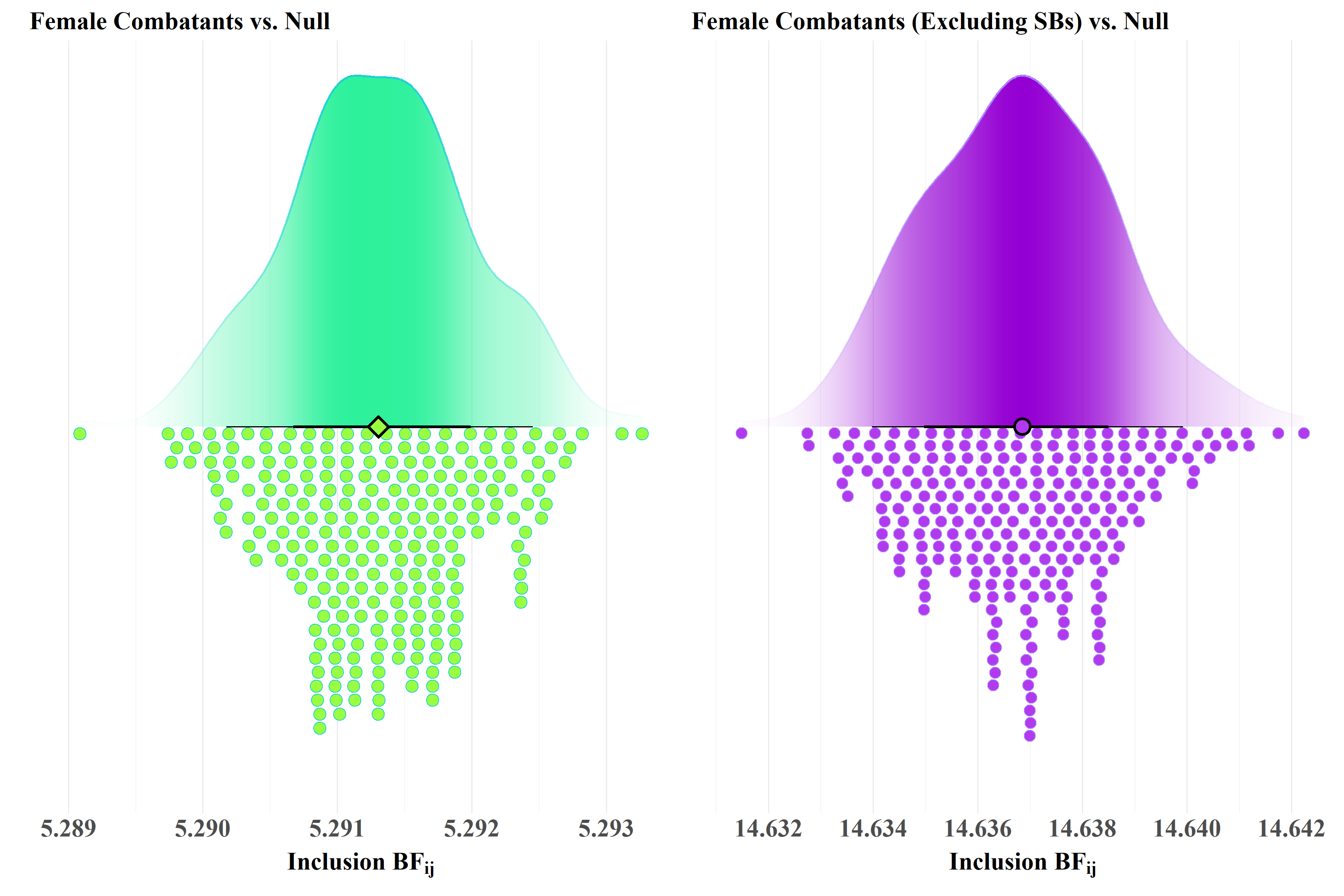
Figure 3: Inclusion Bayes Factors for Female Combatants
Given the prior assumptions about the universe of effect sizes possible and prior probabilities for the hypothesis that rebel groups in which women participate in combat during wartime are more likely to transition to political parties at wars end, the posterior inclusion probability for female combatants is approximately 0.841 when we include cases in which women only participated as suicide bombers and 0.936 if we code participation only in cases where women served in a combat capacity that was not explicitly limited to suicide bombing. Stated differently, as the inclusion Bayes Factors in figure 3 illustrate, the observed data is between 5.29 and 14.64 times more likely to have arisen from those models that include a predictor for female combatants depending on whether we consider cases in which women only participated in combat as suicide bombers or not. This suggests a resonable degree of evidence in support the of the expectation that women’s participation in combat has a small to moderate effect on the probability of rebel to party transitions.
Model Averaged Marginal Effects
Turning to the substantive effect estimate, I illustrate here three different approaches to estimating model averaged marginal effects. When fitting each of the models in the Stan program above, we applied Bayesian g-formula to estimate the population average treatment effect in each of the models containing the female combatants predictor and we can retreive those directly from the brmsfit objects. The model_averaged_ame function shown below implements the approach to averaging over a matrix of posterior probability weights outlined in equation 8 along with the simpler approach from equation 7.
#' Estimating Model Averaged Marginal Effects and Contrasts for Bayesian Models#' #' This function facilitates the estimation of model averaged and stacked #' marginal effects for Bayesian models and is designed to account for uncertainty #' in the process of model specification and selection when estimating average #' marginal effects and probability contrasts.#'#' @aliases model_averaged_ame#' #' @import data.table#'#' @param x A datatable of posterior draws for the average marginal effects#' or predictions such as that returned by the `posterior_contrasts` function.#'#' @param weights An \eqn{n \times m} matrix of posterior probability weights #' such as that returned by `bridgesampling::post_prob` or an m length vector#' of stacking or pseudo-BMA weights.#' #' @param summary A logical argument indicating whether to return the full #' draws for each row in `weights` or return the average for each model-draw #' pair. Defaults to `FALSE`##' @param ... Additional arguments for future development, currently unused.#'#' @return A datatable containing a weighted average of the posterior draws #' for the model averaged marginal effects.#' #' @export model_averaged_ame#' model_averaged_ame<-function(x, weights, ndraws, summary=TRUE, ...){# Nest the draws data framedraws<-x[, list(x.yz =list(.SD)), by=model]# If weights are a matrix, calculate the draws by rowif(is.matrix(weights)){# Construct a matrix of draw weightsweighted_draws<-apply(weights, MARGIN =1, FUN =function(x){brms:::round_largest_remainder(x*ndraws)})# Initialize a list to store the draws inout<-list()# Loop over each column in the matrixfor(iin1:ncol(weighted_draws)){# Randomly sample n rows for each model based on the weightsdraw_ids<-lapply(weighted_draws[, i], function(x){sample(sum(weighted_draws[,i]), size =x)})# Randomly sample n draws proportional to the weightsout[[i]]<-lapply(seq_along(draws[, x.yz]), function(id){draws[, x.yz[[id]][draw_ids[[id]]]]})# Bind the draws into a single data table per repetitionout[[i]]<-rbindlist(out[[i]], idcol ="model")}# Combine everything into a single data tableout<-rbindlist(out, idcol ="bridge_rep")# Average over the bridge sampling repetitions by drawif(isTRUE(summary)){out=out[ , keyby =.(.draw, model),lapply(.SD, mean), .SDcols =patterns("EY|AME")]}}elseif(is.vector(weights)){# Construct a vector of draw weightsweighted_draws<-brms:::round_largest_remainder(weights*ndraws)# Randomly sample n rows for each model based on the weightsdraw_ids<-lapply(weighted_draws, function(x){sample(sum(weighted_draws), size =x)})# Randomly sample n draws proportional to the weightsout<-lapply(seq_along(draws[, x.yz]), function(id){draws[, x.yz[[id]][draw_ids[[id]]]]})# Combine everything into a single data tableout<-rbindlist(out, idcol ="model")}# Return the model averaged drawsreturn(out)}
# Set the seed here for reproducibilityset.seed(2023)# Extract the AMEs from the models containing femrebelsfemrebels_ame_boot<-map( .x =with(params_pos_df, bayes_model_fits[which(femrebels_pos==TRUE)]),~.x$predictions)%>%# Append the list of data tables into onerbindlist(., idcol ="model")# Posterior Probabilities for female rebel modelsfemrebels_bma_marglik<-with(params_pos_df,main_marglik[which(femrebels_pos==TRUE)])# Matrix of Relative Posterior Probabilities for BMAfemrebels_bma_post_probs<-do_call("post_prob", args =unname(femrebels_bma_marglik), pkg ="bridgesampling")# Apply model names to the matrixcolnames(femrebels_bma_post_probs)<-names(femrebels_bma_marglik)# Calculate the weighted draws for each modelfemrebels_bmame<-model_averaged_ame(femrebels_ame_boot, weights =femrebels_bma_post_probs, ndraws =30e3, summary =TRUE)# Print the first few rowshead(femrebels_bmame)
# Extract the AMEs from the models containing femrebels (excluding SBs)femrebels_exs_ame_boot<-map( .x =with(params_pos_df, bayes_model_fits[which(femrebelsexs_pos==TRUE)]),~.x$predictions)%>%# Append the list of data tables into onerbindlist(., idcol ="model")# Posterior Probabilities for female rebel (excluding SBs) modelsfemrebels_exs_bma_marglik<-with(params_pos_df,main_marglik[which(femrebelsexs_pos==TRUE)])# Matrix of Relative Posterior Probabilities for BMAfemrebels_exs_bma_post_probs<-do_call("post_prob", args =unname(femrebels_exs_bma_marglik), pkg ="bridgesampling")# Apply model names to the matrixcolnames(femrebels_exs_bma_post_probs)<-names(femrebels_exs_bma_marglik)# Calculate the weighted draws for each modelfemrebels_exs_bmame<-model_averaged_ame(femrebels_exs_ame_boot, weights =femrebels_exs_bma_post_probs, ndraws =30e3, summary =TRUE)# Print the first few rowshead(femrebels_exs_bmame)
We can then plot the posterior distribution of the BMAMEs using ggdist as shown below which allows us to nicely depict the uncertainty in the estimates. As 4 illustrates, the model averaged marginal effect estimates for the expected difference in the probability of former combatant group transitioning to a post-conflict political party is positive for both measures. When considering only cases where women served in a combat capacity that was not explicitly limited to suicide bombing, we see a 98.38% probability of the effect being positive and in the expected direction with a posterior median of 0.2232 and 89% credible interval spanning the range 0.0625 and 0.3750.
The results are largely identical for the other measure that includes those cases in which female combatants only served as suicide bombers as instances of participation, with a 96.32% probability of the effect being positive and a posterior median of of 0.1875 and an 89% probability the parameter value falls between 0.0268 and 0.3482. Overall, the general conclusion here is rebel groups where women particpate in combat roles during wartime are more likely to form parties and compete in post-conflict elections.
Code
# Append these into a single dataframe for plottingbmame_boot_ests<-rbindlist(list("Female Combtants (Excluding SBs)"=femrebels_exs_bmame, "Female Combtants (Including SBs)"=femrebels_bmame), idcol ="plot_row")# Initialize the ggplot2 object for the model averaged AMEsggplot(bmame_boot_ests, aes(y =AME, x =plot_row))+# Violin plot looking thingsstat_eye(aes( slab_alpha =after_stat(pdf), slab_fill =stat(y>0), point_fill =plot_row, shape =plot_row), slab_size =2, fill_type ="gradient", point_interval ="median_qi", .width =c(0.68, 0.89), point_size =6, stroke =2, show.legend =FALSE, scale =0.7)+# Adjust the y axis scalescale_y_continuous( breaks =scales::pretty_breaks(n =10), limits =c(-0.4, 0.65))+# Adjust fill scalescale_fill_manual( values =c("#23C3E4FF", "#C82803FF"), aesthetics ="slab_fill")+# Adjust fill scalescale_fill_manual( values =c("#3AA2FCFF", "#FD8A26FF"), aesthetics ="point_fill")+# Adjust shape scalescale_shape_manual(values =c(22, 21))+# Add labels to the plotlabs( y =parse(text ="bold('Model Averaged AME '*Delta)"), x ="")
Figure 4: Model Averaged Marginal Effects and Expectations for the Effect of Female Combatants on the Probability of Post-Conflict Party Transitions
Although this is the ideal approach since it accounts for the additional source of computational uncertainty introduced by approximating the marginal likelihood, it can be expensive in terms of both computational time and memory requirements in addition to requiring a minimal knowledge of Stan. We can sidestep Stan and focus exclusively on brms by defining a simple R function to calculate contrasts and model averaged marginal effects as shown below. As figure 5 illustrates, the estimates here are virtually identical and do not differ substantively from those in figure 4. This estimation process is reasonably straightforward and can be used for any model supported by brms.
#' Posterior Contrasts for Bayesian Models fit with {brms}#'#' @param models A named list of model objects of class `brmsfit` for which to #' generate predictions.#' #' @param X A string indicating the name of the treatment in the models.#' #' @param data Data used to fit the model objects.#' #' @param contrasts Values of `X` at which to generate predictions. Defaults to#' `c(0, 1)` but could also be set to factor levels.#' #' @param cores Number of cores to use for parallel computation. If cores > 1,#' future::multisession is used to speed computation via `{furrr}`. Requires#' the `{furrr}` package.#' #' @param ... Additional arguments passed down to `brms::posterior_predict`#'#' @return A list of posterior contrasts for each model in `models`#' #' @export posterior_contrasts#'posterior_contrasts<-function(models, X, data,contrasts=c(0, 1),cores=1,...){# Check that all elements of models are of class brmsfitfor(iinseq_along(models)){brms_check<-brms::is.brmsfit(models[[i]])stopifnot("All elements in models must be of class brmsfit"=brms_check, brms_check)}# Y_i(X = 0, Z)lo<-data|>mutate("{X}":=contrasts[1])# Y_i(X = 1, Z)hi<-data|>mutate("{X}":=contrasts[2])# Check if cores > 1if(cores>1){# Requires {furrr}require(furrr)# Fit models in parallel via futureplan(tweak(multisession, workers =cores))# Posterior predictions for each data setpredictions<-furrr::future_map( .x =models,~.get_posterior_predictions(hi, lo, model =.x, ...), .options =furrr::furrr_options( scheduling =1, seed =TRUE, prefix ="prefix"), .progress =TRUE)# Close the future sessionplan(sequential)}if(cores==1){# Posterior predictions for each data setpredictions<-purrr::map( .x =models,~.get_posterior_predictions(hi, lo, model =.x, ...))}# Return the list of predictionsreturn(predictions)}# Helper function to get posterior prediction contrasts.get_posterior_predictions<-function(hi, lo, model, ...){# Predictions for Y_i(X = 1, Z)EYX1<-brms::posterior_predict(model, newdata =hi, ...)# Predictions for Y_i(X = 0, Z)EYX0<-brms::posterior_predict(model, newdata =lo, ...)# Average over the observations for each draw in the prediction matrixout<-data.table( EYX1 =rowMeans(EYX1), EYX0 =rowMeans(EYX0), AME =rowMeans(EYX1-EYX0), .draw =1:ndraws(model))# Return just the average contrastreturn(out)}
# Models containing femrebelsfemrebels_mods<-with(params_pos_df,bayes_model_fits[which(femrebels_pos==TRUE)])# Generate posterior expectations for the AMEsfemrebels_ame_draws<-posterior_contrasts( models =femrebels_mods, X ="femrebels", data =femrebels_mods[[1]]$data, contrasts =c(0, 1), cores =4)# Calculate the weighted draws for each modelfemrebels_bmame_draws<-model_averaged_ame(femrebels_ame_draws, weights =femrebels_bma_post_probs, ndraws =30e3, summary =TRUE)# Print the first few rowshead(femrebels_bmame_draws)
# Models containing femrebelsfemrebels_exs_mods<-with(params_pos_df,bayes_model_fits[which(femrebelsexs_pos==TRUE)])# Generate posterior expectations for the AMEsfemrebels_exs_ame_draws<-posterior_contrasts( models =femrebels_exs_mods, X ="femrebels_exs", data =femrebel_exs_mods$M112$data, contrasts =c(0, 1), cores =4)# Calculate the weighted draws for each modelfemrebels_exs_bmame_draws<-model_averaged_ame(femrebels_exs_ame_draws, weights =femrebels_exs_bma_post_probs, ndraws =30e3, summary =TRUE)# Print the first few rowshead(femrebels_exs_bmame_draws)
femrebels_bmame_plot_alt<-femrebels_bmame_draws|># Initialize the ggplot2 object for the model averaged AMEggplot(aes(x =AME))+# Add a slab interval to plot the weighted posteriorstat_halfeye(aes( slab_alpha =after_stat(pdf), slab_fill =stat(x>0)), slab_size =2, slab_colour ="#1BD0D5FF", shape =22, fill_type ="gradient", point_interval ="median_qi", .width =c(0.68, 0.89), point_size =6, stroke =2, point_fill ="#99FE42FF", show.legend =FALSE)+# Add labels to the plotlabs( x =parse(text ="bold('Model Averaged AME '*Delta)"), y ="Posterior Density", title ="Female Combtants (Including Suicide Bomber Roles)")+# Adjust fill scalescale_fill_manual( values =c("#208820", "#0060B0"), aesthetics ="slab_fill")+# Adjust the x axis scalescale_x_continuous( breaks =scales::pretty_breaks(n =10), limits =c(-0.4, 0.68))+# Adjust the y axis scalescale_y_continuous(breaks =scales::pretty_breaks(n =6))femrebels_exs_bmame_plot_alt<-femrebels_exs_bmame_draws|># Initialize the ggplot2 object for the model averaged AMEggplot(aes(x =AME))+# Add a slab interval to plot the weighted posteriorstat_halfeye(aes( slab_alpha =after_stat(pdf), slab_fill =stat(x>0)), slab_size =2, slab_colour ="#1BD0D5FF", shape =22, fill_type ="gradient", point_interval ="median_qi", .width =c(0.68, 0.89), point_size =6, stroke =2, point_fill ="#99FE42FF", show.legend =FALSE)+# Add labels to the plotlabs( x =parse(text ="bold('Model Averaged AME '*Delta)"), y ="Posterior Density", title ="Female Combtants (Excluding Suicide Bomber Roles)")+# Adjust fill scalescale_fill_manual( values =c("#208820", "#0060B0"), aesthetics ="slab_fill")+# Adjust the x axis scalescale_x_continuous( breaks =scales::pretty_breaks(n =10), limits =c(-0.4, 0.68))+# Adjust the y axis scalescale_y_continuous(breaks =scales::pretty_breaks(n =6))(femrebels_bmame_plot_alt/femrebels_exs_bmame_plot_alt)
Figure 5: Model Averaged Marginal Effects and Expectations for the Effect of Female Combatants on the Probability of Post-Conflict Party Transitions, Direct Estimation
Illustration in {marginaleffects}
Finally, in the interest of encouraging applied researchers to take uncertainty seriously and integrate sensitivity analysis into their work directly rather than treating it as something to undertake only when forced, I turn now to a straightforward illustration of BMAMEs using the marginaleffects package which provides the necessary functionality to handle most of the above steps automatically thanks to the feature-rich support for various approaches to averaging across posterior distributions provided by brms.
To obtain the BMAME for a given parameter while accounting for the uncertainty in the model specifications, version 0.5.0 and higher of marginaleffects allows users to specify the argument type = "average" in their call to either marginaleffects::marginaleffects or marginaleffects::comparisons for objects of class brmsfit along with any additional arguments to be passed down to pp_average such as the type of weights to estimate, or alternatively a numeric vector of pre-estimated weights which is usually the more computationally efficient option and the approach I take in the example below.
Although up to this point I have been averaging over all possible combinations of models containing the parameter of interest, we will take a step back here and focus on the full model specifications, averaging over two models that differ only in which of the female combatants measures they contain. I begin by specifying and estimating each of the models using brms.
# Prepare the data, we need the two variables to be named the samemodel_data<-list("femrebels"=model_df%>%mutate(femrebel =femrebels),"femrebels_exs"=model_df%>%mutate(femrebel =femrebels_exs))# Model formula for the female rebels modelsfemrebel_bf<-bf(elect_party~femrebels+left_ideol+nationalist+un_intervention+party_affil+ethnic_group+un_intervention+africa+qsi_pol+qsi_econ+qsi_social)# Specify priors for the model parametersfemrebel_logit_priors<-prior(normal(0, 0.75), class =b)+prior(normal(0, 1), class =Intercept)# Define the custom stanvars for the bootstrapped g-formula for comparison purposesgformula_vars<-stanvar( x =1, name ="treat_pos", block ="data", scode ="int<lower = 1, upper = K> treat_pos; // Treatment Position")+# Code for the transformed data blockstanvar( scode =" // Bootstrap Probabilities vector[N] boot_probs = rep_vector(1.0/N, N); // Matrices for the bootstrapped predictions matrix[N, Kc] Xa; matrix[N, Kc] Xb; // Potential Outcome Y(X = 1, Z) Xa = X[, 2:K]; Xa[, treat_pos] = ones_vector(N); // Potential Outcome Y(X = 0, Z) Xb = X[, 2:K]; Xb[, treat_pos] = zeros_vector(N); ", position ="end", block ="tdata")+# Code for the bootstrapped g-formula in generated quantitiesstanvar( scode =" // Row index to be sampled for bootstrap int row_i; // Calculate Average Marginal Effect in the Bootstrapped sample real AME = 0; array[N] real Y_X1; // Potential Outcome Y(X = 1, Z) array[N] real Y_X0; // Potential Outcome Y(X = 0, Z) for (n in 1:N) { // Sample the Baseline Covariates row_i = categorical_rng(boot_probs); // Sample Y(x) where x = 1 and x = 0 Y_X1[n] = bernoulli_logit_rng(b_Intercept + Xa[row_i] * b); Y_X0[n] = bernoulli_logit_rng(b_Intercept + Xb[row_i] * b); // Add Contribution of the ith Observation to the Bootstrapped AME AME = AME + (Y_X1[n] - Y_X0[n])/N; } // Take the mean of the posterior expectations real EYX1 = mean(Y_X1); // E[Y | X = 1, Z] real EYX0 = mean(Y_X0); // E[Y | X = 0, Z] ", position ="end", block ="genquant")
# Fit each of the models (6 chains, 8k iterations), takes about 3 secondsfemrebels_logit_fits<-map2( .x =model_data, .y =str_c("Party_Transition_Logit_", names(model_data), ".rds"), .f =~brm( formula =femrebel_bf, family =brmsfamily("bernoulli", link ="logit"), prior =femrebel_logit_priors, data =.x, cores =12, # Max number of cores to use for parallel chains chains =6, # Number of chains, should be at least 4 iter =8000, # Total iterations = Warm-Up + Sampling warmup =3000, # Warm-Up Iterations stanvars =gformula_vars, # Custom Stan code to include in the model save_pars =save_pars(all =TRUE), seed =2023, backend ="cmdstanr", sample_prior ="yes", file =.y))# Add PSIS LOO-CV and Marginal Likelihoodfemrebels_logit_fits<-map( .x =femrebels_logit_fits, .f =~add_criterion(.x, criterion =c("loo", "marglik"), max_iter =5e3, repetitions =25, cores =8, silent =TRUE))
We can then use bridgesampling::post_prob to obtain the relative probability of each model based on the marginal likelihood estimates and brms::loo_model_weights to obtain cross-validation based stacking and pseudo-BMA weights. We can then use comparisons to estimate the model averaged probability contrasts.
# Get the posterior probability weightspostprob_weights<-bridgesampling::post_prob(femrebels_logit_fits[[1]]$criteria$marglik, # Full Model, Including Suicide Bombersfemrebels_logit_fits[[2]]$criteria$marglik, # Full Model, Excluding Suicide Bombers prior_prob =c(0.5, 0.5), # This is the default, I'm just being explicit model_names =c("femrebels", "femrebels_exs"))# Calculate Pseudo-BMA+ Weightspbma_weights<-loo_model_weights(femrebels_logit_fits[[1]],femrebels_logit_fits[[2]], method ="pseudobma", model_names =names(femrebels_logit_fits), BB =TRUE, # Pseudo-BMA+ with Bayesian Bootstrap BB_n =10000, # Use 10k replications for Bayesian Bootstrap cores =8L)# Calculate Stacking Weightsstacking_weights<-loo_model_weights(femrebels_logit_fits[[1]],femrebels_logit_fits[[2]], method ="stacking", model_names =names(femrebels_logit_fits), optim_control =list(reltol =1e-10), cores =8L)# Store all the weights in a named listweights_ls<-list("BMA"=apply(postprob_weights, 2, mean),"Stacking"=stacking_weights,"Pseudo-BMA+"=pbma_weights)# Print a comparison of the weightsprint(weights_ls)
# Calculate model averaged contrastscomparisons_femrebels<-map( .x =weights_ls,~comparisons(femrebels_logit_fits[[1]], m1 =femrebels_logit_fits[[2]], # Subsequent models must be named arguments variables ="femrebel", type ="average", transform_pre ="differenceavg", weights =.x, method ="posterior_predict"# Accounts for observation-level uncertainty))# Extract the posterior drawscomparisons_femrebels_draws<-map( .x =comparisons_femrebels,~posteriordraws(.x, shape ="long"))# Bind the draws frames into a data tablecomparisons_femrebels_draws<-rbindlist(comparisons_femrebels_draws, idcol ="type")
Figure 6 shows a side by side comparison of the weighted average of the contrasts based on different weighting approaches. The results here are largely the same as those above, but we have combined the two measures into a single model-wise mixture distribution and can incorporate what is effectively measurement uncertainty here directly into the quantity of interest. The marginaleffects implementation is somewhat limted by its dependence on brms::pp_average and it is on my list of things to do for the coming year to work out a more efficient approach that allows for the efficiency and flexibility of those illustrated in the preceding section.
Code
# Initialize the ggplot2 object for the model averaged AMEscomparisons_femrebels_draws%>%ggplot(aes(y =draw, x =weights))+# Violin plot looking thingsstat_eye(aes( slab_alpha =after_stat(pdf), slab_fill =weights, point_fill =weights, shape =weights), slab_size =2, fill_type ="gradient", point_interval ="median_qi", .width =c(0.68, 0.89), point_size =6, stroke =2, show.legend =FALSE, scale =0.8)+# Adjust the y axis scalescale_y_continuous( breaks =scales::pretty_breaks(n =10), limits =c(-0.19, 0.54))+# Adjust fill scalescale_fill_manual( values =c("#23C3E4FF", "#C82803FF", "#2EF19CFF"), aesthetics ="slab_fill")+# Adjust fill scalescale_fill_manual( values =c("#3AA2FCFF", "#FD8A26FF", "#99FE42FF"), aesthetics ="point_fill")+# Adjust shape scalescale_shape_manual(values =c(22, 21, 24))+# Add labels to the plotlabs( y =parse(text ="bold('Model Averaged AME '*Delta)"), x ="")
Figure 6: Model Averaged Marginal Effects for the Effect of Female Combatants on the Probability of Post-Conflict Party Transitions, {marginaleffects} Implementation
Conclusion
This concludes what was hopefully a detailed illustration of model averaged marginal effects with brms, marginaleffects, and Stan. The general takeaway here is that selecting a single model is usually the wrong approach and there is seldom any need to do so. While no method of estimation is perfect, BMA and its variants provide a principled, relatively robust way to propagate uncertainty in quantities typically of interest to researchers in the social sciences and can help us avoid unnecessary dichotomies that are, in most cases, false. By applying probability theory to average across posterior distributions when estimating average marginal effects, we can obtain interpretable model averaged estimates for both linear and non-linear regression models.
As far as subsequent developments are concerned, this is effectively the cornerstone of my dissertation work so I am hoping to have at least one subsequent post illustrating and implementing BMAMEs for multilevel models that employ non-linear link functions in the comining weeks. In the meantime, however, remember that nothing good ever comes from mixing odds and ratios or exposing your relatives to unnecessary risks and holding the random effects in a hierarchical model at their mean still gives you a conditional estimate that results in a weak connection between theory and data. Finally, if you catch any mistakes–and I can almost guarentee there are many in a post of this length–either leave a comment or let me know some other way (i.e., twitter).
Cranmer, Skyler J., Douglas R. Rice, and Randolph M. Siverson. 2015. “What to Do about Atheoretic Lags.”Political Science Research and Methods 5(4): 641–65.
Hollenbach, Florian M., and Jacob M. Montgomery. 2020. “Bayesian Model Selection, Model Comparison, and Model Averaging.” In The SAGE Handbook of Research Methods in Political Science and International Relations, eds. Luigi Curini and Robert Franzese. SAGE Publications Ltd, 937–60.
For a recent application of BMA in the context of instrument selection see Rozenas and Zhukov (2019).↩︎
It is entirely possible this is wrong and does not actualy make sense so if someone has a better idea or suggestions for improvements I would love to hear them.↩︎
There is no such thing as an “uninformative prior”; the concept itself is not mathematically defined.↩︎
As Plümper and Traunmüller (2018) demonstrate, BMA performs quite well in terms of this latter objective.↩︎
Those familiar with the post-conflict rebel parties literature in political science are likely rolling their eyes at this sentence because in its present state it is not clear we know much of anything about causal relationships.↩︎
Estimation is performed under Stan version 2.30.1 on a desktop computer with a Ryzen 9 5900X CPU and 128GB of DDR4 memory.↩︎
One might contrast this with frequentist p-values in the NHST framework common in the social sciences which answer the question under the simplifying assumption the null hypothesis is true, what is the probability of observing a result more extreme than the one we did? Although still widely taught, this provides a very precise answer to a question few researchers are interested in and rejecting the strawman null that the effect of \(\mathrm{X}\) is exactly equal to zero–something no respectable researcher actually believes–tells you nothing about your vaguely defined alternative (Gill 1999; Gross 2014).↩︎
This is only in part because I can’t figure out the correct brms::do_call syntax to pass both a list of marglik objects and model priors to bridgesampling::post_prob.↩︎
---title: An Introduction to Being Less Wrongsubtitle: Bayesian Hypothesis Testing and Model Averaged Marginal Effects for the Social Sciencespagetitle: An Introduction to Being Less Wrongdate: 2022-12-31description: "This post provides an introduction to Bayesian Model Averaging and Model Averaged Marginal Effects with Stan, `{brms}`, and `{marginaleffects}`"categories: [R, Bayesian Statistics, Statistics, Marginal Effects, Stan, Logit, Model Averaging]license: All content in this post is made available for public use under a Creative Commons Attribution-ShareAlike 4.0 International (CC BY-SA 4.0) License.image: figs/fig-model-averaged-ame-margins.svgtoc-location: leftpage-layout: fullcode-fold: true# Execution optionsexecute: freeze: true# Social Media Informationopen-graph: title: "An Introduction to Being Less Wrong" description: "Bayesian Hypothesis Testing and Model Averaged Marginal Effects for the Social Sciences" image: "figs/bmame-blog-post-preview.png"twitter-card: title: "An Introduction to Being Less Wrong" image: "figs/bmame-blog-post-preview.png" card-style: summary_large_image description: "Bayesian Hypothesis Testing and Model Averaged Marginal Effects for the Social Sciences" creator: "@adamjnafa" site: "@adamjnafa"---```{r setup, include=FALSE}knitr::opts_chunk$set(cache =FALSE,warning =FALSE,message =FALSE,comment =' ',fig.path ='figs/',fig.align ="center",fig.process =function(x) { x2 =sub('-\\d+([.][a-z]+)$', '\\1', x)if (file.rename(x, x2)) x2else x })# Load the necessary librariespacman::p_load("tidyverse", "arrow","data.table","brms", "furrr", "cmdstanr","patchwork","ggdist","marginaleffects",install =FALSE)# Custom theme for data visualizationsplot_theme <-function(title_size =NULL, xaxis_size =NULL, yaxis_size =NULL, strip_size =NULL, strip_face =NULL, caption.hjust =1, caption.vjust =0, x_axis_face =NULL, y_axis_face =NULL, transparent =FALSE, axis_text_size =NULL, legend_text_size =NULL,subtitle_size =NULL,caption_size =NULL,base_size =12, ...) { .theme <-theme_minimal(base_size = base_size) +theme(# Specify the default settings for the plot titleplot.title =element_text(size = title_size,face ="bold",family ="serif" ),# Specify the default settings for caption textplot.caption =element_text(size = caption_size,family ="serif",hjust = caption.hjust,vjust = caption.vjust ),# Specify the default settings for subtitle textplot.subtitle =element_text(size = subtitle_size,family ="serif" ),# Specify the default settings specific to the x axis titleaxis.title.y =element_text(size = yaxis_size, face = y_axis_face, family ="serif",margin =margin(r =10, l =-10) ),# Specify the default settings specific to the y axis titleaxis.title.x =element_text(size = xaxis_size, face = x_axis_face, family ="serif",margin =margin(t =10, b =-10) ),# Specify the default settings for x axis textaxis.text.x =element_text(size = axis_text_size,family ="serif",face = x_axis_face ),# Specify the default settings for y axis textaxis.text.y =element_text(size = axis_text_size,family ="serif",face = y_axis_face ),# Specify the default settings for legend titleslegend.title =element_text(size = legend_text_size,face ="bold",family ="serif" ),# Specify the default settings for legend textlegend.text =element_text(size = legend_text_size,family ="serif" ),# Set the strip background fill to blankstrip.background =element_blank(),# Adjust the strip text size settingsstrip.text =element_text(family ="serif", size = strip_size,face = strip_face ),# Additional Settings Passed to theme() ... )# Plot Transparencyif (transparent ==TRUE) { .theme <- .theme +theme(panel.background =element_rect(fill ="transparent", colour =NA),plot.background =element_rect(fill ="transparent", colour =NA),legend.background =element_rect(fill ="transparent", colour =NA),legend.key =element_rect(fill ="transparent", colour =NA) ) }return(.theme)}## Set the base theme settings for ggplot2theme_set(plot_theme(xaxis_size =24,yaxis_size =24,title_size =24,caption_size =24,axis_text_size =24,strip_face ="bold",y_axis_face ="bold",x_axis_face ="bold",plot.margin =margin(2, 2, 4, 5, "mm"),plot.caption.position ="plot",plot.title.position ="plot",strip_size =24,legend_text_size =24,legend.position ="top",caption.hjust =0, caption.vjust =-1,transparent =TRUE ))```# IntroductionGeorge E. P. Box famously described the problem of model development in statistics and related fields by noting, *all models are wrong, but some are useful* [-@Box1976]. That is, all models are necessarily simplifications of a much more complex reality and statistics is by no means an algorithmic truth generating process because no model can ever be true in the pure sense of the word. Yet, this at times underappreciated reality does not render all models useless but rather implies the goal of those who practice statistics in its various forms is to develop and identify models that are useful in a never ending quest to be less wrong. In this post I introduce an approach to this task that has been the subject of my own dissertation work on the use of Bayesian Model Averaging (BMA) to account for uncertainty in model specification when estimating average marginal effects in non-linear regression models. ::: a I outline here what I term a Bayesian Model Averaged Marginal Effect (BMAME) in the context of logistic regression models in political science and illustrate how to obtain BMAMEs in a straightforward manner using the `{marginaleffects}` R package [@ArelBundock2022a], which thanks to Vincent Arel-Bundock's assistance supports model averaged orstacked average marginal effects for any model fit with the Stan interface `{brms}`[@Burkner2017; @Burkner2018]. I also provide a more general demonstration in Stan that makes the method easily applicable in Python and high dimensional settings. Although I focus here on models that include only population-level effects, recent feature additions to `{marginaleffects}` now make it possible to obtainBMAMEs from more complex hierarchical models and I will cover such applications in a subsequent post.::: # Bayesian Model Averaging in Political ScienceAlthough Bayesian Model Averaging was introduced to political science more than two decades ago by @Bartels1997, cases of its use in applied work remain rare and are largely confined to the topic of political methodology [@Juhl2019; @Cranmer2015; @Montgomery2010].[^1] This presents something of a problem given the numerous studies demonstrating the dangers of tossing a large number of likely correlated predictors into a regression model [@Achen2005; @Clarke2005; @Clarke2009; @Montgomery2018]; the reality that if we wish to adjudicate between two or more competing theories, comparing coefficients in a single model is generally insufficient to accomplish such a task [@Imai2011; @Clarke2007; @Hollenbach2020]; and the difficulty of assessing what we truly known about political phenomenon that results from an obsession with "statistical significance" and precise answers to poorly defined questions [@Ward2010; @Schrodt2014; @Lundberg2021]. [^1]: For a recent application of BMA in the context of instrument selection see @Rozenas2019.::: a In minor contrast to the past advice of @Montgomery2010 who suggest "BMA is best used as a subsequent robustness check to show that our inferences are not overly sensitive to plausible variations in model specification" (266), I argue here model averaging can and should be used as far more than a robustness check if forno other reason than a model-wise mixture distribution for the paramter of interest is almost certainly more informative than a point estimate from a single model specification. Indeed, BMA providesone of the few natural and intuitive ways of resolving some of the issues outlined in the preceding paragraph, particularly as it pertains to the evaluation of non-nested theoretical models, while alsoexhibiting a lower false positive rate than alternative approaches [@Pluemper2018]. This section provides a brief explanation of BMA and its connection to model averaged marginal effects before proceeding to a discussion of how the procedure is implemented.::: ## Bayesian Model Comparison and Model AveragingConsider a simple case in which we have a set of $\mathcal{M}$ models, each of which characterizes a possible representation of some unknown data generation process. Although it remains common practice in applied political science to select a single model based on a largely arbitrary fit statistic (i.e., AIC, $\chi^{2}$, or whatever people are getting a p-value from this week), such an approach is problematic since it ignores the uncertainty inherent in the process of model specification. Rather than selecting a single model and consequently placing an implicit zero prior on **every other possible model specification you could have reasonably considered but did not**, Bayesian Model Averaging and its analogues provide a means of averaging across several possible, potentially non-nested, model specifications and accounting for the uncertainty associated with doing so.::: a Imagine we wish to adjudicate between two competing theoretical models in the set of candidate models $\mathcal{M}$. The posterior odds of model $i$ relative to an alternative $k$ can be expressed as:::$$\underbrace{\frac{\Pr(\mathcal{M}_{i} \, | \, y)}{\Pr(\mathcal{M}_{k} \, | \, y)}}_{\mathrm{Posterior~Odds}} = \underbrace{\frac{p(y \, | \, \mathcal{M}_{i})}{p(y \, | \, \mathcal{M}_{k})}}_{\mathrm{Bayes~Factor}} \times \underbrace{\frac{\pi(\mathcal{M}_{i})}{\pi(\mathcal{M}_{k})}}_{\mathrm{Model~Prior}}$$ {#eq-posterior-odds} where $\pi(\mathcal{M})$ is the prior probability of model $i$ over model $k$ and $p(y \,|\, \mathcal{M})$ is the marginal likelihood of the observed data under each of the candidate models such that$$\underbrace{p(y \,|\, \mathcal{M})}_{\mathrm{Marginal~Likelihood}} = \int\underbrace{p(y \,|\, \theta,\, \mathcal{M})}_{\mathrm{Likelihood}} \, \underbrace{\pi(\theta \,|\, \mathcal{M})}_{\mathrm{Prior}}d\theta$$ {#eq-marginal-likelihood}::: a Given our prior assumptions about how likely the observed data are to have arisen from each model in the set $\mathcal{M}$, the result of equation @eq-posterior-odds is the posterior odds of model $i$ compared to model $k$ and thus captures the relative probability that model $\mathcal{M_{i}}$ represents the true data generation process compared to the plausible alternative $\mathcal{M_{k}}$. We can easily extend this example to the setting in which $\mathcal{M_{k}}$ is a set of plausible competing models of size $k > 2$, in which case the posterior model probability of the $i^{th}$ model relative to each of the alternatives $k$ is:::$$\Pr(\mathcal{M}_{i} \,|\, y) = \frac{p(y \, | \, \mathcal{M}_{i}) \, \cdot \, \pi(\mathcal{M}_{i})}{\displaystyle\sum^{\mathcal{m}}_{k=1} p(y \, | \, \mathcal{M}_{k}) \, \cdot \, \pi(\mathcal{M}_{k})}$$ {#eq-posterior-probability} Applying equation @eq-posterior-probability to each model in the set under consideration yields a vector of relative posterior model probabilities of length $m$ which may be used as either posterior probability weights as in the case of Bayesian Model Averaging or for the estimation of posterior inclusion probabilities.::: a In the context of model averaging, we can take draws from the posterior predictive distribution of each model containing a given parameter of interest proportional to its posterior probability weight obtained from equation @eq-posterior-probability. This yields a model-wise mixture representing a weighted average of the posterior predictive distribution for some parameter such as a regression coefficient for a linear model or as I outline below, an average marginal effect or probability contrast for models that employ a non-linear link function. ::: ## Bayesian Model Averaged Marginal EffectsAverage marginal effects are ubquitous in the social sciences though, as [Andrew Heiss nicely illustrates](https://www.andrewheiss.com/blog/2022/05/20/marginalia/), the term average marginal effect is often used ambiguously and in the context of more complex models, the terms marginal andconditional [tend to be a source of additional confusion](https://www.andrewheiss.com/blog/2022/11/29/conditional-marginal-marginaleffects/). In the case of a simple population-level linear model with a Gaussian likelihood and identity link function, the model averaged marginal effect is equivalent to the posterior distribution of the model averaged coefficient $\beta$ which can be expressed as$$\mathbb{E}(\beta \, | \, y) = \sum_{i=1}^{m}\Pr(\mathcal{M}_{i} \, | \, y) \cdot \mathbb{E}(\beta\, |\, \mathcal{M}_{i}, \, y) \quad \forall \quad i \in \{1, 2,\dots, m\}$$ {#eq-bma-population} where $\Pr(\mathcal{M}_{i} ~ | ~ y)$ represent the posterior model probability and $\mathbb{E}(\beta ~|~ \mathcal{M}_{i}, ~ y)$ is the expected value of some parameter $\beta$ conditional on the observed data and some model specification for each model $i$ in the set of models under consideration $m$ [@Montgomery2010].::: aFor probability models such as logit, and other commonly used formulations for modelingdiscrete responses, this simple closed form solution does not exist nor is there any meaningfulway to interpret the coefficients of these models as efffect size estimates--a reality that unfortunately remains quite widely misunderstood [@Mood2009; @Daniel2020]. As a general principle, **any model morecomplex than a simple linear regression can only be meaningfully interpreted in terms of the predictionsit generates** [@Long2018], which in the case of logistic regression simply means applying the inverse logistic function to obtain predicted probabilities which we can then use to estimate contrasts or average marginal effects [@Norton2019]. Letting $\mathrm{Y}$ represent a binary outcome, $\mathrm{X}$ a continuous exposure or treatment of interest, and $\mathrm{Z}$ a matrix of measured confounders, we can express the average marginal effect as:::$$\mathrm{AME}\Delta_{j} = \int \frac{\mathbb{E}[\mathrm{Y}_{ij} ~ | ~ \mathrm{X}_{ij} = \mathrm{x}_{ij} + h, \mathrm{Z}_{ij}] ~-~ \mathbb{E}[\mathrm{Y}_{ij} ~ | ~ \mathrm{X}_{ij} = \mathrm{x}_{ij}, \mathrm{Z}_{ij}]d\mathrm{Z}}{h} \\$$ {#eq-logit-continuous-ame} which provided a sufficiently small value of $h$, yields a reasonable approximation of the partial derivative and provides a posterior distribution for the average effect of an instantaneous change in $\mathrm{X}$ on theprobability scale similar to what one obtains in linear regression.::: aSimilarly, for a binary treatment of interest we apply the Bayesian g-formula to obtain the average marginal effect of $\mathrm{X}$ on the probability of $\mathrm{Y}$ as shown in equation @eq-logit-binary-ame.:::$$\mathrm{AME}\Delta_{j} = \int \mathbb{E}[\mathrm{Y}_{ij} ~ | ~ \mathrm{X}_{ij} = 1, \mathrm{Z}_{ij}] ~-~ \mathbb{E}[\mathrm{Y}_{ij} ~ | ~ \mathrm{X}_{ij} = 0, \mathrm{Z}_{ij}]d\mathrm{Z} \\$$ {#eq-logit-binary-ame}Equations @eq-logit-continuous-ame and @eq-logit-binary-ame make clear we are averaging over the confounder distribution $\mathrm{Z}$ rather than holding it constant at some fixed value [@Oganisian2020; @Keil2017]. This point is an important one because in binary outcome models such as logit and probit, holding $\mathrm{Z}$ constant at some fixed value such as the mean corresponds to **an entirely different estimand** [@Hanmer2012].The AME is a population-averaged quantity, corresponding to the population average treatment effect and thesetwo quantities can produce very different results under fairly general conditions because **they do not answer the same question**.::: aFrom here it is straightforward to obtain a model averaged marginal effect estimate for a discrete outcome modelsuch as logit. Given marginal predictions for each model $k$ in the set $m$, we can apply equation @eq-logit-binary-bmame to obtain the posterior distribution of average marginal effects for each model.:::$$\begin{align}\mathrm{BMAME}\Delta_{j} &= \sum_{k=1}^{m} \Pr(\mathcal{M}_{k} | y)\cdot\int \mathbb{E}[\mathrm{Y}_{ij}, \mathcal{M}_{k} | \mathrm{X}_{ij} = 1, \mathrm{Z}_{ij}] ~-~ \mathbb{E}[\mathrm{Y}_{ij}, \mathcal{M}_{k} | \mathrm{X}_{ij} = 0, \mathrm{Z}_{ij}]d\mathrm{Z} \\&= \sum_{k=1}^{m} \Pr(\mathcal{M}_{k} | y)\cdot\mathrm{AME}\Delta_{k,j}\end{align}$$ {#eq-logit-binary-bmame} This yields a model-wise mixture distribution representing the weighted average of the marginal effectsestimates and has broad applicability to scenarios common in the social sciences, industry, and any other setting where a need arises to account for uncertainty in model specification.## Limitations and CaveatsWhile traditional marginal likelihood-based Bayesian model averaging is a powerful and principled technique for dealing with uncertainty in the process of model specification and selection, it is not without limitations and caveats of its own, some of which bear emphasizing before proceeding further.### Marginal Likelihood and Computational UncertaintyFirst, for all but the simplest of models attempting to derive the integral in equation @eq-marginal-likelihood analytically proves to be computationally intractable and we must instead rely on algorithmic approximations such as bridge sampling [@Gronau2017; @Gelman1998; @Wang2020].While the bridge sampling approximation tends to perform well compared to common alternatives,estimates of the marginal likelihood $p(y \,|\, \mathcal{M})$ may be highly variable upon repeated runs of the algorithm [@Schad2022]. This problem tends to arise in morecomplex hierarchical models with multiple varying effects and, perhaps unsurprisingly, suggeststhat by relying on approximations we introduce an additional source of computational uncertainty that may need to be accounted for.::: aFor the purposes of BMAMEs, I have elsewhere proposed addressing this additional source of uncertainty and incorporating it into the estimates by executing the bridge sampling algorithm $S$ times for each model to obtain a distribution of possible values for the approximate log marginal likelihood. Given a vector of estimates for $p(y ~|~ \mathcal{M})$ of length $s$ for each model $k \in \{1,2,\dots, m\}$, we can apply equation @eq-posterior-probability to obtain an $s \times m$ matrix of posterior model probabilities. It is then straightforward to extend equation @eq-logit-binary-bmame to average over the distribution of posterior probability weights rather than relying on single estimate or point estimate as shown in equation @eq-logit-bmame-reps below.[^2]$$\begin{align}\mathrm{BMAME}\Delta_{j} &=\frac{1}{S}\sum_{s=1}^{S} \left[\sum_{k=1}^{m} \Pr(\mathcal{M}_{k, s} | y)\cdot\int \mathbb{E}[\mathrm{Y}_{ij}, \mathcal{M}_{k} | \mathrm{X}_{ij} = 1, \mathrm{Z}_{ij}] ~-~ \mathbb{E}[\mathrm{Y}_{ij}, \mathcal{M}_{k} | \mathrm{X}_{ij} = 0, \mathrm{Z}_{ij}]d\mathrm{Z}\right]\\&= \frac{1}{S}\sum_{s=1}^{S}\left[\sum_{k=1}^{m} \Pr(\mathcal{M}_{k, s} | y)\cdot\mathrm{AME}\Delta_{k,j}\right]\end{align}$$ {#eq-logit-bmame-reps} Whether this approach is necessary depends largely on how variable the algorithm is on repeated runsand it may simply be adequate to instead take the median or mean of the marginal likelihood estimates foreach model. Although it is beyond the scope of this post, one could also use exhaustive leave-future-out cross-validation which is equivalent to the marginal likelihood given a logarithmic scoring rule [@Fong2020; @Buerkner2020], though this approach tends to be extremely expensive in terms of computation.:::[^2]: It is entirely possible this is wrong and does not actualy make sense so if someone has a better idea or suggestions for improvements I would love to hear them.### Bayes Factors and Prior SensitivityThe second caveat with respect to obtaining BMAMEs stems from a common criticism of Bayes Factors. Althoughas the amount of available data $n \longrightarrow \infty$, the likelihood will tend to dominate the prior in Bayesian estimation, this is not necessarily the case in terms of inference. Indeed, from equations @eq-marginal-likelihood and @eq-posterior-probability one can quite clearly see the the posterior probability $\Pr(\mathcal{M} ~| ~y)$ depends on the prior probability of the parameters, $\pi(\theta \,|\, \mathcal{M})$ in equation @eq-marginal-likelihood, and the respective prior probability $\pi(\mathcal{M})$ of each model in the set under consideration. Since our substantive conclusions may be sensitive to either of these prior specifications, these assumptions should be checked to verify the results do not vary wildly under reasonable alternatives. ::: aPerhaps more importantly, due to their dependence on Bayes Factors, posterior probability weights require atleast moderatlely informative priors on each and every parameter in a model and it is by this point common knowledge that specifying a flat or "uninformative" prior such as $\beta \sim \mathrm{Uniform(-\infty, \infty)}$ or even an excessively vague one tends to bias Bayes Factors--and by extension values that depend on them--violently in favor of the null model.[^3] This is a feature of applied Bayesian inference rather than abug and **if you make stupid assumptions, you will arrive at stupid conclusions**. The solution to this problem is to think carefully about the universe of possible effect sizes you might observe for a given parameter, assign reasonable priors that constrain the parameter space, and verify the results are robust to alternative distributional assumptions.[^3]: There is no such thing as an "uninformative prior"; the concept itself is not mathematically defined.:::::: {.callout-caution collapse="true"}### Likeihoods and PriorsThe degree to which a prior can be considered informative is heavily dependent on the likelihood and can often only be understood in that context [@Gelman2017].:::### Stacking, and the Open-$\mathcal{M}$ ProblemFinally, traditional BMA is flawed in the sense that its validity rests upon the closed $\mathcal{M}$ assumption implicit in equation @eq-posterior-probability. In the open $\mathcal{M}$ setting where the true model is not among those in the set of candidate models under consideration, as will generally be the case in any real world application, estimated effects based on posterior probability weights are likely to be biased [@Hollenbach2020; @Yao2018]. This problem arises from the fact that marginal-likelihood based posterior probability weights for each model $m \in \mathcal{M}$ correspond to the probability a given model captures the true data generation process and in most settings this is unlikely to ever be the case since, by definition, *all models are wrong*. ::: aIn the open $\mathcal{M}$ setting, traditional BMA will still assign each model some probability but since by definition $\sum_{i=1}^{m}\Pr(\mathcal{M}_{i} ~|~ y) = 1$, these weights no longer have a valid interpretation in terms of the posterior probability a given model is true. Although this does not render marginal likelihood based model averaging useless and it may often make more sense to think about model specification and selection as a probabilistic process aimed at identifying the most likely model conditional on the set of models under consideration [@Hinne2020], it is advisable to assess whether our substantive conclusions are sensitive to potential violations of the closed $\mathcal{M}$ assumption. This once again underscores the fact that statistics is not a mechanistic truth generating process and *there is no magic*. It also underscores the need to think in more local terms--rather than asking *is this model true* we generally want to know *the probability $\mathrm{X}$ belongs to the true data generation process*.[^4][^4]: As @Pluemper2018 demonstrate, BMA performs quite well in terms of this latter objective.An alternative but still properly Bayesian approach aimed at addressing these potential flaws in traditional BMA is cross-validation based stacking [@Yao2018]. In contrast to traditional BMA, stacking and pseudo-BMA weights are constructed based on the relative expectation of the posterior predictive density [@Hollenbach2020; @Yao2018]. These approaches to estimating model weights do not rely upon the closed $\mathcal{M}$ assumption, and thus provide a way of either avoiding it altogether or relaxing it as a robustness check on the posterior probability weights, albeit while answering a fundamentally different question more appropriate for an open $\mathcal{M}$ world. Since the overall approach to calculating model averaged AMEs does not changeand we are merely substituting the posterior probability weights in equation @eq-logit-binary-bmame withstacking or pseudo-BMA weights, I direct readers to @Yao2018 for a formal discussion of these approaches.::: # Female Combatants and Post-Conflict Rebel PartiesTo illustrate the utility of BMAMEs in political science, I draw on an example adapted from the second chapter ofmy dissertation in which I examine how the active participation of women in rebel groups during wartime shapes the political calculus of former combatant groups at war's end. In short, I expect rebel groups where women participate in combat roles during wartime to be *more likely* to form political parties and participate in post-conflict elections. ## DataTo identify the universe of post-conflict successor parties to former combatant groups I rely on the Civil War Successor Party (CWSP) dataset which includes all civil wars in the UCDP Armed Conflicts Dataset (UCDP) that terminated between 1970 and 2015 [@Daly2020]. Since the primary distinction between political parties and other civil society organizations such as interest groups lies in the latter's participation in elections and fielding candidates for political office and a party that does not compete in elections is no party at all, I operationalize our dependent variable, *Rebel to Party Transition*, as a binary event which takes a value of 1 if a rebel group both forms a political party and directly participates in a country's first post-conflict elections and 0 otherwise. The resulting sample consists of 112 observations for 108 unique rebel groups across 56 countries, approximately 66% of which formed parties and participated in their country's first post-conflict election.::: aFollowing @Wood2017, I define female combatants as members of a rebel group who are "armed and participate in organized combat activities on behalf of a rebel organization" (38). I code instances of female participation in rebel groups by mapping version 1.4 of the Women in Armed Rebellion Data (WARD) to the CWSP and construct two versions of the main predictor of interest based on the best estimate for the presence of female combatants in a given rebel group, one of which includes cases in which women served only as suicide bombers while the other codes these groups as not having any women in combat positions. Each of these variables takes a value of 1 if women participated in combat in a given rebel group and 0 otherwise. Among the rebel groups in our analysis, female combatants have been active in some capacity in 52.67% of those who were involved in civil wars that have terminated since 1970 and 50.89% featured women in non-suicide bombing roles.I also adjust for several additional factors that may otherwise confound the estimate of the effect of female participation in combat on rebel successor party transitions. First, insurgent groups that attempt to perform functions typically characteristic of the state during wartime may be more likely to transition to political parties following the end of a conflict since, in doing so, they both develop organizational capacity and if successful, demonstrate that they are capable of governing to their future base of support. Moreover, as rebel groups build organizational capacity and accumulate institutional knowledge, their ability to sustain a successful insurgency and recruit combatants grows as well. To adjust for rebel organizational capacity I specify a Bayesian multidimensional item response model to construct a latent scale capturing the degree to which rebel groups engaged in functions of the state during wartime based on twenty-six items from Quasi-State Institutions dataset [@Albert2022].Second, I adjust for baseline characteristics of each rebel group that previous research suggests influences both where women rebel and post-conflict party transitions. Drawing on data from @Braithwaite2019, I construct a series of dichotomous indicator variables for whether a rebel group is affiliated with an existing political party [@Manning2016], nationalist and left-wing or communist ideological origins [@Wood2017], and whether a group has ties to a specific ethnic community since this may provide advantages in terms of mobilizing combatants and voters along specific cleavages. I also construct two additional indictators to capture whether the United Nations intervened in the conflict and whether a given rebel group was located in Africa.While it is, of course, impossible in the context of an observational setting such as this one to isolateevery possible source of confounding, nor is it generally advisable to attempt to do so, I focus on these baseline covariates since existing research provides a strong theoretical basis to suspect they impact the relationship of interest.[^5] For the purposes of this illustration, I assume this set of covariatesis sufficient to satisfy strong ignorability but such an assumption is likely unreasonable and the particular analysis here may ultimately best be taken as descriptive in nature.:::[^5]: Those familiar with the post-conflict rebel parties literature in political science are likely rolling their eyes at this sentence because in its present state it is not clear we know much of anything about causal relationships.```{r}# Load the required librariespacman::p_load("tidyverse", "arrow","data.table","brms", "furrr", "cmdstanr","patchwork","ggdist","marginaleffects",install =FALSE)# Read in the pre-processed datamodel_df <-read_parquet("data/model_data.gz.parquet")```## Model and PriorsTo estimate the effect of women's participation in combat on post-conflict rebel party transitions for this example, I specify a simple logit model as shown in equation @eq-logit-model. The bernoulli probability $\mu$ of a rebel group transitioning to a political party at war's end is modeled as a function of the population-level intercept $\alpha$ and a vector of coefficients $\beta_{k}$ corresponding to the matrix of inputs $X_{n}$.$$\begin{align}y_{i} &\sim \mathrm{Bernoulli}(\mu)\\\mathrm{logit}(\mu) &= \alpha + X_{n}\beta_{k}\\\text{with priors}\\\alpha &\sim \mathrm{Normal}(0, 1)\\\beta_{k} &\sim \mathrm{Normal}(0, 0.75)\end{align}$$ {#eq-logit-model}::: aSince we model $\mu$ via a logit link function, our priors on the intercept $\alpha$ and coefficients $\beta_{k}$ should correspond to the expected change in the log odds of the response for each predictor. Some may find the process of prior elicitation in logistic regression models difficult since reasoning on the logit scale may seem unintuitive. As figure @fig-logit-scaleillustrates, the the log odds of the response for models with that employ a logit link function is effectively bounded between approximately $-6$ and $6$. Values in excess of $|5|$ generally should not occur unless your data exhibits near complete or quasi-complete separation.:::```{r fig-logit-scale, echo = TRUE, dev='svg'}#| label: fig-logit-scale#| fig-width: 14#| fig-height: 12#| fig-align: center#| fig-dpi: 300#| fig-cap: "Scale of the Logit Link"#| ## Simulate logit probabilitieslogit_scale <-tibble(x =seq(-6.5, 6.5, 0.0001),y = brms::inv_logit_scaled(x))## Plot the logit scaleggplot(logit_scale, aes(x = x, y = y)) +## Add a line geomgeom_line(size =3, color ="firebrick") +## Add labelslabs(x ="Log Odds", y ="Probability") +## Adjust the x axis scale breaksscale_x_continuous(breaks =seq(-6, 6, 1)) +## Adjust the y axis scale breaksscale_y_continuous(breaks =seq(0, 1, 0.1))```::: aFramed in terms of effect sizes, a change of $\pm 3$ in the log odds of the response relative to the baseline spans half the logit scale in either direction. In the social sciences where data is largely random noise and effect sizes are typically small to moderate at best and while the road to hell is paved with *rules of thumb*, we can generally assume *a priori* that 1) any true effect of a given parameter $\beta$ in the population is likely modest in magnitude and 2) values closer zero are more likely than those further away. From these relatively straightforward assumptions, we can arrive at a prior for the coefficients that follows a normal distribution with mean 0 and scale $0.75$ as shown in equation @eq-logit-model. In practical terms, this assumes the universe possible effect sizes for each predictor is normally distributed in the range of approximately $-1.5$ and $1.5$ on the logit scale. For the population-level intercept $\alpha$ I assign a slightly more diffuse normal prior mean 0 and scale 1 or $\alpha \sim \text{Normal}(0,~1)$ which reflects a slightly greater degree of uncertainty about the baseline probability but is still moderately informative and constrains the bulk of the prior density in the range of realistic values. It is important to note here that as shown in Stan model below, we are specifying a prior on the intercept for the centered inputs rather than on the original scale. To more explicitly communicate our prior assumptions, we can use the tools for visualizing uncertainty provided in the `{ggdist}` package as shown in figure @fig-logit-priors below [@Kay2022].:::```{r logit-priors-code, echo = TRUE, eval = FALSE}# Simulate the prior probabilitieslogit_priors <-tibble(alpha_prior =rnorm(10e5, 0, 1),beta_prior =rnorm(10e5, 0, 0.75)) %>%## Pivot the simulated data to long formpivot_longer(everything())# Set parameter names for the facets----logit_prior_labels <-as_labeller(x =c("beta_prior"="bolditalic(beta[k] * phantom(.) * phantom() %~% phantom() * phantom(.) * Normal(0*list(,) * phantom(.) * 0.75))","alpha_prior"="bolditalic(alpha[k] * phantom(.) * phantom() %~% phantom() * phantom(.) * Normal(0*list(,) * phantom(.) * 1))" ), default = label_parsed)# Plot the prior distributionslogit_prior_plots <- logit_priors %>%# Initiate the ggplot objectggplot(aes(x = value, fill = name, shape = name)) +# Facet by the prior distributionsfacet_wrap(~ name, scales ="free", labeller = logit_prior_labels) +# Add a half eye geom for the prior distributionsstat_halfeye(aes(slab_alpha =stat(pdf)),.width =c(.68, .95),fill_type ="gradient",show.legend =FALSE ) +# Manually set the fill colorsscale_fill_manual(values =c("#208820", "#0060B0")) +# Manually set the shapesscale_shape_manual(values =c(22, 24)) +# Adjust the breaks on the y axisscale_x_continuous(breaks = scales::pretty_breaks(n =8)) +# Add labels to the plotlabs(y ="Prior Probability Density",x = latex2exp::TeX(r'(Log $\Pr(\theta_{prior})$)', bold = T) )# Plot back transformed probabilitiesprob_trans_plots <- logit_priors %>%# Initiate the ggplot objectggplot(aes(fill = name, shape = name)) +# Facet by the prior distributionsfacet_wrap(~ name, scales ="free", labeller = logit_prior_labels) +# Add a half eye geom for the prior distributionsstat_halfeye(aes(x =plogis(value), slab_alpha =stat(pdf)),.width =c(.68, .95),fill_type ="gradient",show.legend =FALSE ) +# Manually set the fill colorsscale_fill_manual(values =c("#208820", "#0060B0")) +# Manually set the shapesscale_shape_manual(values =c(22, 24)) +# Add labels to the plotlabs(y ="Prior Probability Density",title ="",x = latex2exp::TeX(r'($\Pr(\theta_{prior})$)', bold =TRUE) ) +# Adjust the breaks on the x axisscale_x_continuous(breaks = scales::pretty_breaks(n =8))## Print the combined plotlogit_prior_plots/prob_trans_plots``````{r, echo = FALSE}#| label: fig-logit-priors#| fig-align: center#| fig-cap: "Priors for the Logit Model Parameters"knitr::include_graphics("figs/Prior_Probs_S2.png")```::: aSince the model here is computationally quite efficient--on average, each model takes approximately 2.5 seconds to converge with 30,000 post-warmup draws--and in the interest of completeness, I search the full parameter space which consists of $2^{k}$ possible model specifications. Although it is possible to do this in this context, researchers will often instead need to place constrain the number of possible model configurations, generally by specifying an implicit prior model probability of 1 for certain parameters [@Montgomery2010; @Hinne2020]. Although `{brms}` provides an easy to use R interface to Stan that makes fitting a wide variety of Bayesian regression models easier than ever before and requires no direct knowledge of Stan, it is limited for my purposes here by the fact that it requires recompiling the underlying Stan model for each fit. This process ends up being extremely inefficient for a large number of model configurations since each model takes three times as long to compile as it does to fit.To circumvent this issue, I implement the model directly in Stan in a way designed to be directly compatible with `{brms}`. For models containing the parameter of interest, the model implments the bayesian g-formula to estimate the average marginal effect of women's participation in combat on the probability of a rebel-to-party transition during the estimation process in the generated quanitites block. As I previously demonstrated in [this post](../statistical-adjustment-interpretation/index.qmd), it is then possible to compile the Stan model once and use the same program for each dataset using `{cmdstanr}` directly. Further computational gains can be obtained by using the `{furrr}` package to fit multiple models in parallel and I specify a series of functions to streamline this process as shown below.:::::: panel-tabset### g-formula```stan// Bayesian Logit Model with Optional Bootstrapped AMEs via the Bayesian g-formuladata { int<lower=1> N; // N Observations array[N] int Y; // Response Variable int<lower=1> K; // Number of Population-Level Effects matrix[N, K] X; // Population-level Design Matrix int prior_only; // Should the likelihood be ignored? int treat_pos; // Data for the bootstrapped AMEs}transformed data { int Kc = K - 1; matrix[N, Kc] Xc; // centered version of X without an intercept vector[Kc] means_X; // column means of X before centering for (i in 2 : K) { means_X[i - 1] = mean(X[ : , i]); Xc[ : , i - 1] = X[ : , i] - means_X[i - 1]; } // Bootstrap Probabilities vector[N] boot_probs = rep_vector(1.0/N, N); // Matrices for the bootstrapped predictions matrix[N, Kc] Xa; matrix[N, Kc] Xb; // Potential Outcome Y(X = 1, Z) Xa = X[, 2:K]; Xa[, treat_pos - 1] = ones_vector(N); // Potential Outcome Y(X = 0, Z) Xb = X[, 2:K]; Xb[, treat_pos - 1] = zeros_vector(N);}parameters { vector[Kc] b; // Regression Coefficients real Intercept; // Centered Intercept}transformed parameters { real lprior = 0; // Prior contributions to the log posterior lprior += normal_lpdf(b | 0, 0.75); lprior += normal_lpdf(Intercept | 0, 1);}model { // likelihood including constants if (!prior_only) { target += bernoulli_logit_glm_lpmf(Y | Xc, Intercept, b); } // priors including constants target += lprior;}generated quantities { // Actual population-level intercept real b_Intercept = Intercept - dot_product(means_X, b); // Additionally sample draws from priors array[Kc] real prior_b = normal_rng(0, 0.75); real prior_Intercept = normal_rng(0, 1); // Row index to be sampled for bootstrap int row_i; // Calculate Average Marginal Effect in the Bootstrapped sample real AME = 0; array[N] real Y_X1; // Potential Outcome Y(X = 1, Z) array[N] real Y_X0; // Potential Outcome Y(X = 0, Z) for (n in 1:N) { // Sample the Baseline Covariates row_i = categorical_rng(boot_probs); // Sample Y(x) where x = 1 and x = 0 Y_X1[n] = bernoulli_logit_rng(b_Intercept + Xa[row_i] * b); Y_X0[n] = bernoulli_logit_rng(b_Intercept + Xb[row_i] * b); // Add Contribution of the ith Observation to the Bootstrapped AME AME = AME + (Y_X1[n] - Y_X0[n])/N; } // Take the mean of the posterior expectations real EYX1 = mean(Y_X1); // E[Y | X = 1, Z] real EYX0 = mean(Y_X0); // E[Y | X = 0, Z]}```### Reference```stan// Bayesian Logit Model for Models without the Treatment Variabledata { int<lower=1> N; // total number of observations array[N] int Y; // response variable int<lower=1> K; // number of population-level effects matrix[N, K] X; // population-level design matrix int prior_only; // should the likelihood be ignored?}transformed data { int Kc = K - 1; matrix[N, Kc] Xc; // centered version of X without an intercept vector[Kc] means_X; // column means of X before centering for (i in 2 : K) { means_X[i - 1] = mean(X[ : , i]); Xc[ : , i - 1] = X[ : , i] - means_X[i - 1]; }}parameters { vector[Kc] b; // Regression Coefficients real Intercept; // Centered Intercept}transformed parameters { real lprior = 0; // Prior contributions to the log posterior lprior += normal_lpdf(b | 0, 0.75); lprior += normal_lpdf(Intercept | 0, 1);}model { // likelihood including constants if (!prior_only) { target += bernoulli_logit_glm_lpmf(Y | Xc, Intercept, b); } // priors including constants target += lprior;}generated quantities { // Actual population-level intercept real b_Intercept = Intercept - dot_product(means_X, b); // Additionally sample draws from priors array[Kc] real prior_b = normal_rng(0, 0.75); real prior_Intercept = normal_rng(0, 1);}```### Functions```r#' A Function for building combinations of formulas for model averaging#' #' @importFrom glue glue_collapse#' @importFrom purrr map_chr#' @importFrom stringr str_replace#'#' @param terms A named list of terms to create all unique combinations of.#' See usage example for direction on how to specify each term#' #' @param resp A string specifying the name of the response vector#' #' @param base_terms An optional argument indicating additional terms to#' include in all formulas. This can be used to place implicit constraints on #' the parameter space to reduce computational burden#' #' @param ... Reserved for future development but currently#' unused#'#' @return A character vector of model formulas containing all unique #' combinations of the elements in terms#' #' @export bma_formulas#' #' @examples#' # Specify the input for the resp argument#' response <- "fun"#' #' # Specify the inputs for the terms argument#' covariates <- list(#' age = c("", "age"),#' sex = c("", "sex"),#' rock = c("", "rock")#' )#' #' # Build the formulas#' model_forms <- bma_formulas(terms = covariates, resp = response)#' bma_formulas <-function(terms, resp, base_terms =NULL, ...) {## Validate the formula argumentsstopifnot(exprs = {is.list(terms)is.character(resp) })## Make a list of all unique combinations of lhs ~ rhs formulas <-expand.grid(terms, stringsAsFactors =FALSE)## Initialize a list to store the formulas in out <-list()## Build a list of formulas for each pair formulasfor (i in1:nrow(formulas)) { out[[(i)]] <-glue_collapse( formulas[i, !is.na(formulas[i, ])], sep =" + " ) }# Paste the response term out <-paste(resp, "~", out)# If base_terms is non-null, add additional terms to all formulasif (!is.null(base_terms)) { out <-paste(out, base_terms, sep =" + ") } out <-map_chr(.x = out, ~str_replace(.x, "character\\(0\\)", "1") )return(out)}#' Fitting Models in Parallel with brms via cmdstanr#'#' @param formula A `brmsformula` object for the model.#' #' @param treat A string argument containing the name of the treatment#' or a regular expression to match against the columns in `data`.#' #' @param prior A `brmsprior` object containing the priors for the model.#' #' @param data A data frame containing the response and inputs named in#' `formula`.#' #' @param cores The maximum number of MCMC chains to run in parallel.#' #' @param chains The number of Markov chains to run.#' #' @param warmup The number of warmup iterations to run per chain.#' #' @param sampling The number of post-warmup iterations to run per chain.#' #' @param stan_models The compiled Stan program(s) to be passed to #' `cmdstanr::sample`.#' #' @param save_file The file path where the brmsfit object should be saved.#' #' @param ... Additional arguments passed to `brms::brm`#'#' @return An object of class `brmsfit`#' #' @export cmdstan_logit#'cmdstan_logit <-function(formula, treat, prior, data, cores, chains, warmup, sampling, stan_models, save_file, ...) {# Check if the file already exists file_check <-file.exists(save_file)if (isTRUE(file_check)) {# Read in the file if it already exists out <- readr::read_rds(file = save_file) } else {# Total iterations for brms niter <- sampling + warmup# Initialize an empty brmsfit object brms_obj <-brm(formula = formula,family =brmsfamily("bernoulli", link ="logit"),prior = prior,data = data,cores = cores,chains = chains,iter = niter,warmup = warmup,empty =TRUE,seed =123456,sample_prior ="yes", ... )# Get the data for the stan model stan_data <-standata(brms_obj)# Check whether the model contains the treatment stan_data$treat_pos <-.match_treat_args(stan_data, treat)# Select the Stan model to use based on the dataif (!is.null(stan_data$treat_pos)) { cmdstan_model <- stan_models[["gformula"]] } else { cmdstan_model <- stan_models[["reference"]] }# Fit the brms model out <-.fit_cmdstan_to_brms(cmdstan_model, brms_obj, stan_data, cores, chains, warmup, sampling)# Write the brmsfit object to an rds file readr::write_rds(out, file = save_file, "xz", compression =9L) }# Return the model objectreturn(out)}# Function for detecting the treatment vector.match_treat_args <-function(stan_data, treat) {# Check if any of the columns in X match the treatment check_treat <-grepl(treat, colnames(stan_data$X))# Get the position of the treatment if presentif (any(check_treat)) { treat_pos <-which(check_treat) } else { treat_pos <-NULL }return(treat_pos)}# Function to fit the models with cmdstanr and store them in the empty brmsfit.fit_cmdstan_to_brms <-function(cmdstan_model, brms_obj, stan_data, cores, chains, warmup, sampling) {# Set the initial number of draws to 0 min_draws <-0# Repeat the run if any of the chains stop unexpectedlywhile (min_draws < (sampling * chains)) {# Fit the Stan Model fit <- cmdstan_model$sample(data = stan_data,seed =123456,refresh =1000,sig_figs =5,parallel_chains = cores,chains = chains,iter_warmup = warmup,iter_sampling = sampling,max_treedepth =13 )# Update the check min_draws <- posterior::ndraws(fit$draws()) }# Convert the environment to a stanfit object and add it to the brmsfit brms_obj$fit <- rstan::read_stan_csv(fit$output_files())# Rename the parameters brms_obj <- brms::rename_pars(brms_obj)# Store the expectations inside the brmsfit objectif (!is.null(stan_data$treat_pos)) {# Extract the expectations and contrasts brms_obj$predictions <- fit$draws(variables =c("EYX0", "EYX1", "AME"), format ="draws_df" ) }# Store run times brms_obj$times <- fit$time()# Return the brmsfit objectreturn(brms_obj)}```:::::: aWe can then generate a formula for each of the $2^{k}$ model combinations, specify priors, and compile the Stan programs to be passed to `cmdstan_logit` as shown below. I estimate each of the 384 possible candidate models,running six parallel markov chains for iterations 8,000 each and discarding the first 3,000 after the initial warmup adaptation stage.[^6] This leaves 30,000 post-warmup draws per model for post-estimation inference. While this is well in excess of what is required for reliable estimation, the large number of samples is necessary to ensure stability of the bridge sampling approximation for the marginal likelihood [@Schad2022]. Fitting three models in parallel via `{furrr}`, estimation and approximate leave one out cross validation take less than 10 minutes in total to complete. Oweing in part to the fact I run the algorithm 250 times per model, however, the run time to estimate the marginal likelihood via bridge sampling takes roughly 9 hours in total.:::[^6]: Estimation is performed under Stan version 2.30.1 on a desktop computer with a Ryzen 9 5900X CPU and 128GB of DDR4 memory.::: panel-tabset### Preparation```r# Define the list of predictors, parameter space is 2^kmodel_terms <-list(femrebels =c("femrebels", "femrebels_exs", NA),left_ideol =c("left_ideol", NA),nationalist =c("nationalist", NA),un_intervention =c("un_intervention", NA),party_affil =c("party_affil", NA),ethnic_group =c("ethnic_group", NA),africa =c("africa", NA),qsi =c("qsi_pol + qsi_econ + qsi_social", NA))# Build the model formulas, results in 383 combinationsmodel_forms <-bma_formulas(terms = model_terms, resp ="elect_party") %>%map(.x = ., ~bf(.x))# Specify priors for the model parameterslogit_priors <-prior(normal(0, 0.75), class = b) +prior(normal(0, 1), class = Intercept)# Names of the files to write the models tofits_files <-str_c( main_priors_dir,"Party_Transition_Logit_Main_",seq_along(model_forms),".rds")# Compile the Stan modelsbayes_logit_mods <-list("reference"=cmdstan_model(stan_file =str_c( main_priors_dir, "Party_Transition_Logit_Main.stan" ), force_recompile =FALSE ),"gformula"=cmdstan_model(stan_file =str_c( main_priors_dir, "Party_Transition_Logit_Main_gformula.stan" ), force_recompile =FALSE ))```### Estimation```r# Planning for the futureplan(tweak(multisession, workers =3))# Fit the models in parallel via {future}bayes_model_fits <-future_map2(.x = model_forms,.y = fits_files,.f =~cmdstan_logit(formula = .x,prior = logit_priors,treat ="femrebels|femrebels_exs",data = model_df,cores =6,chains =6,warmup =3e3,sampling =5e3,stan_models = bayes_logit_mods,save_file = .y,control =list(max_treedepth =13),save_pars =save_pars(all =TRUE) ),.options =furrr_options(scheduling =1,seed =TRUE,prefix ="prefix" ),.progress =TRUE) # Takes about ~5 minutes in total```### Post-Estimation```r# Add PSIS LOO CV Criteriabayes_model_fits <-future_map2(.x = bayes_model_fits,.y = fits_files,.f =~add_criterion( .x,criterion ="loo",cores =4,file = stringr::str_remove(.y, ".rds") ),.options =furrr_options(scheduling =1,seed =TRUE,prefix ="prefix" ),.progress =TRUE) # Takes about ~4 minutes in total# Add log marginal likelihood----bayes_model_fits <-future_map(.x = bayes_model_fits,.f =~add_criterion( .x,criterion ="marglik",max_iter =5e3,repetitions =250,cores =8,silent =TRUE ),.options =furrr_options(scheduling =1,seed =TRUE,prefix ="prefix" ),.progress =TRUE) # Takes about ~9.5 hours in total# Back from the futureplan(sequential)```::: ## Hypothesis TestingIn a Bayesian framework, model comparison is formalized by means of posterior model probabilities as shown in equation @eq-posterior-probability. Given $m$ possible candidate models and letting $i$ denote those containing the parameter of interest and $k$ those that do not, we can obtain posterior *inclusion* and *exclusion* probabilities for a given parameter. The ratio of these two probabilities shown in equation @eq-inclusion-prob is an inclusion Bayes Factor and represents the relative posterior odds of models containing the parameter of interest compared to all of the candidate models that do not.$$\mathrm{BF_{Inclusion}}~=~\frac{\sum_{i=1}\Pr(\mathcal{M}_{i} \, | \, y)}{\sum_{k=1}\Pr(\mathcal{M}_{k} \, | \, y)}$$ {#eq-inclusion-prob}::: aIn terms of hypothesis testing, posterior inclusion probabilities provide the *epistemologically correct* way to answer the questions most social science studies are concerned with--given our modeling assumptions, howlikely are those models containing the treatment $\mathrm{X}$ compared to those that do not. In other words, a posteriorinclusion probability provides a continuous measure of evidence we can use to evaluate how probable it is ourtreatment or intervention of interest belongs to the true data generation process [@Hinne2020].[^7]Although my interest here lies primarily in using the posterior model probabilities to obtain a model-wise mixture distribution of the substantive effect estimates, I breifly illustrate how one can formally test a hypothesis in a Bayesian framework and obtain a vague answer to a precise question. This may be useful in a sequential testingapproach where we first wish to evaluate whether an effect exists before preceding to interpretation though onemay also simply assume effects exist and focus on estimating their magnitude instead.For the purposes of this illustration, I compare those models containing each of the two measures of women's participation in combat during civil wars to each of the possible model specifications that does not include either of the two measures. Although by convention, it is common to take the prior model probabilities to beequally likely--in effect an implicit uniform prior--this is far from the only possible approach and in manycases, particularly when adjudicating between competing theories, it may make more sense to weight the hypothesesaccording to some external source such as existing research on the subject, meta-analyses, etc. For simplicityhere, I assume each of the models is equally likely a priori and obtain posterior probabilities and inclusion Bayes Factors for the parameters of interest as shown below.[^8]:::[^7]: One might contrast this with frequentist p-values in the NHST framework common in the social sciences which answer the question *under the simplifying assumption the null hypothesis is true, what is the probability of observing a result more extreme than the one we did?* Although still widely taught, this provides a very precise answer to a question few researchers are interested in and rejecting the strawman null that the effect of $\mathrm{X}$ is exactly equal to zero--something no respectable researcher actually believes--tells you nothing about your vaguely defined alternative [@Gross2014; @Gill1999].[^8]: This is only in part because I can't figure out the correct `brms::do_call` syntax to pass both a list of marglik objects *and* model priors to `bridgesampling::post_prob`.::: panel-tabset### Preparation```r# Extract the parameters of interest in each modelmodel_params <-map( bayes_model_fits, ~variables(.x) %>%str_subset(., "^b_"))# Build a reference data frame with the positions of the predictorsparams_pos_df <-tibble(# Model Namesmodel =str_c("M", 1:length(model_params)),# Female Rebels (Including Suicide Bombers)femrebels_pos =map_lgl( model_params,~str_which(.x, "b_femrebels$") %>%length() ==1 ),# Female Rebels (Excluding Suicide Bombers)femrebelsexs_pos =map_lgl( model_params, ~str_which(.x, "b_femrebels_exs") %>%length() ==1 ),# No Female Rebels Predictorreference_pos =map_lgl( model_params, ~str_which(.x, "b_femrebel*") %>%length() %>%!. ))# Apply names to the model fits listnames(bayes_model_fits) <-str_c("M", 1:length(bayes_model_fits))# Extract the marginal likelihood object from each modelmain_marglik <-map(bayes_model_fits, ~ .x$criteria$marglik)```### Female Rebels (Including SBs)```r# Posterior Probabilities for female rebel modelsfemrebels_marglik <-with( params_pos_df, main_marglik[c(which(femrebels_pos ==TRUE),which(reference_pos ==TRUE) )])# Matrix of Relative Posterior Probabilitiesfemrebels_post_probs <-do_call("post_prob", args =unname(femrebels_marglik), pkg ="bridgesampling")# Apply model names to the matrixcolnames(femrebels_post_probs) <-names(femrebels_marglik) # Build a tibble for the comparisonsfemrebels_vs_null_df <-tibble(prob_femrebels =rowSums(femrebels_post_probs[, 1:128]),prob_null =rowSums(femrebels_post_probs[, 129:255]),Inclusion_BF = prob_femrebels/prob_null)```### Female Rebels (Excluding SBs)```r# Posterior Probabilities for female rebel models (excluding SBs)femrebels_exs_marglik <-with( params_pos_df, main_marglik[c(which(femrebelsexs_pos ==TRUE),which(reference_pos ==TRUE) )])# Matrix of Relative Posterior Probabilitiesfemrebels_exs_post_probs <-do_call("post_prob", args =unname(femrebels_exs_marglik), pkg ="bridgesampling")# Apply model names to the matrixcolnames(femrebels_exs_post_probs) <-names(femrebels_exs_marglik) # Build a tibble for the comparisonsfemrebels_exs_vs_null_df <-tibble(prob_femrebels_exs =rowSums(femrebels_exs_post_probs[, 1:128]),prob_null =rowSums(femrebels_exs_post_probs[, 129:255]),Inclusion_BF = prob_femrebels_exs/prob_null)```::: ```{r read-comparisons, echo=FALSE}# Load the comparisons list from diskcomparisons <-read_rds("data/comparisons_moderate_priors_ls.rds")# Posterior Probabilities for female rebel models (including SBs)femrebels_post_probs <- comparisons$femrebels_post_probs# Inclusion Probabilities for female rebel models (excluding SBs)femrebels_vs_null_df <- comparisons$femrebels# Posterior Probabilities for female rebel models (excluding SBs)femrebels_exs_post_probs <- comparisons$femrebels_exs_post_probs# Inclusion Probabilities for female rebel models (excluding SBs)femrebels_exs_vs_null_df <- comparisons$femrebels_exs``````{r fig-bayes-comparisons, echo = TRUE}#| label: fig-comparisons-bayes#| fig-width: 18#| fig-height: 12#| fig-align: center#| fig-dpi: 300#| fig-cap: "Inclusion Bayes Factors for Female Combatants"#| # Fancy ggplots because aestheticsbf_femrebels_vs_null <-ggplot(data = femrebels_vs_null_df, aes(x = Inclusion_BF)) +# Slab stat for the raincloud plotstat_slab(aes(slab_alpha =stat(pdf)),slab_color ="#1BD0D5FF",fill_type ="segments",fill ="#2EF19CFF",show.legend =FALSE,scale =1 ) +# Dot interval stat for the raincloud plotstat_dotsinterval(point_interval ="median_qi",fill ="#99FE42FF",shape =23,.width =c(0.68, 0.90),point_size =6,stroke =2,slab_color ="#1BD0D5FF",show.legend =FALSE,side ="bottom",layout ="weave",dotsize =0.75 ) +# Add axis labelslabs(title ="Female Combatants vs. Null",x =parse(text ="bold(Inclusion~BF[ij])"),y ="" ) +# Adjust the breaks on the x axisscale_y_continuous(breaks =NULL) +# Adjust the breaks on the y axisscale_x_continuous(breaks = scales::pretty_breaks(n =6))# Fancy ggplots because aestheticsbf_femrebels_exs_vs_null <-ggplot(data = femrebels_exs_vs_null_df, aes(x = Inclusion_BF)) +# Slab stat for the raincloud plotstat_slab(aes(slab_alpha =stat(pdf)),slab_color ="#AB82FF",fill_type ="segments",fill ="#9400D3",show.legend =FALSE,scale =1 ) +# Dot interval stat for the raincloud plotstat_dotsinterval(point_interval ="median_qi",fill ="#B23AEE",shape =21,.width =c(0.68, 0.90),point_size =6,stroke =2,slab_color ="#AB82FF",show.legend =FALSE,side ="bottom",layout ="weave",dotsize =0.75 ) +# Add axis labelslabs(title ="Female Combatants (Excluding SBs) vs. Null",x =parse(text ="bold(Inclusion~BF[ij])"),y ="" ) +# Adjust the breaks on the x axisscale_y_continuous(breaks =NULL) +# Adjust the breaks on the y axisscale_x_continuous(breaks = scales::pretty_breaks(n =6))bf_femrebels_vs_null|bf_femrebels_exs_vs_null```::: aGiven the prior assumptions about the universe of effect sizes possible and prior probabilities for the hypothesis that rebel groups in which women participate in combat during wartime are more likely to transition to political parties at wars end, the posterior inclusion probability for female combatants is approximately 0.841 when we include cases in which women only participated as suicide bombers and 0.936 if we code participation only in caseswhere women served in a combat capacity that was not explicitly limited to suicide bombing. Stated differently, as the inclusion Bayes Factors in figure @fig-comparisons-bayes illustrate, the observed data is between 5.29 and 14.64 times more likely to have arisen from those models that include a predictor for female combatants depending on whether we consider cases in which women only participated in combat as suicide bombers or not.This suggests a resonable degree of evidence in support the of the expectation that women's participation in combat has a small to moderate effect on the probability of rebel to party transitions.:::## Model Averaged Marginal EffectsTurning to the substantive effect estimate, I illustrate here three different approaches to estimating model averaged marginal effects. When fitting each of the models in the Stan program above, we appliedBayesian g-formula to estimate the population average treatment effect in each of the models containing the female combatants predictor and we can retreive those directly from the `brmsfit` objects. The`model_averaged_ame` function shown below implements the approach to averaging over a matrix of posteriorprobability weights outlined in equation @eq-logit-bmame-reps along with the simpler approach from equation@eq-logit-binary-bmame.::: panel-tabset### Functions```r#' Estimating Model Averaged Marginal Effects and Contrasts for Bayesian Models#' #' This function facilitates the estimation of model averaged and stacked #' marginal effects for Bayesian models and is designed to account for uncertainty #' in the process of model specification and selection when estimating average #' marginal effects and probability contrasts.#'#' @aliases model_averaged_ame#' #' @import data.table#'#' @param x A datatable of posterior draws for the average marginal effects#' or predictions such as that returned by the `posterior_contrasts` function.#'#' @param weights An \eqn{n \times m} matrix of posterior probability weights #' such as that returned by `bridgesampling::post_prob` or an m length vector#' of stacking or pseudo-BMA weights.#' #' @param summary A logical argument indicating whether to return the full #' draws for each row in `weights` or return the average for each model-draw #' pair. Defaults to `FALSE`##' @param ... Additional arguments for future development, currently unused.#'#' @return A datatable containing a weighted average of the posterior draws #' for the model averaged marginal effects.#' #' @export model_averaged_ame#' model_averaged_ame <-function(x, weights, ndraws, summary =TRUE, ...) {# Nest the draws data frame draws <- x[, list(x.yz =list(.SD)), by=model]# If weights are a matrix, calculate the draws by rowif (is.matrix(weights)) {# Construct a matrix of draw weights weighted_draws <-apply( weights, MARGIN =1, FUN =function(x) { brms:::round_largest_remainder(x * ndraws) })# Initialize a list to store the draws in out <-list()# Loop over each column in the matrixfor (i in1:ncol(weighted_draws)) {# Randomly sample n rows for each model based on the weights draw_ids <-lapply(weighted_draws[, i], function(x){sample(sum(weighted_draws[,i]), size = x) })# Randomly sample n draws proportional to the weights out[[i]] <-lapply(seq_along(draws[, x.yz]), function(id) { draws[, x.yz[[id]][draw_ids[[id]]]] })# Bind the draws into a single data table per repetition out[[i]] <-rbindlist(out[[i]], idcol ="model") }# Combine everything into a single data table out <-rbindlist(out, idcol ="bridge_rep")# Average over the bridge sampling repetitions by drawif (isTRUE(summary)) { out = out[ , keyby = .(.draw, model),lapply(.SD, mean), .SDcols =patterns("EY|AME") ] } } elseif (is.vector(weights)) {# Construct a vector of draw weights weighted_draws <- brms:::round_largest_remainder(weights * ndraws)# Randomly sample n rows for each model based on the weights draw_ids <-lapply(weighted_draws, function(x){sample(sum(weighted_draws), size = x) })# Randomly sample n draws proportional to the weights out <-lapply(seq_along(draws[, x.yz]), function(id) { draws[, x.yz[[id]][draw_ids[[id]]]] })# Combine everything into a single data table out <-rbindlist(out, idcol ="model") }# Return the model averaged drawsreturn(out)}```### Female Rebels (Including SBs)```r# Set the seed here for reproducibilityset.seed(2023)# Extract the AMEs from the models containing femrebelsfemrebels_ame_boot <-map(.x =with( params_pos_df, bayes_model_fits[which(femrebels_pos ==TRUE)] ),~ .x$predictions ) %>%# Append the list of data tables into onerbindlist(., idcol ="model")# Posterior Probabilities for female rebel modelsfemrebels_bma_marglik <-with( params_pos_df, main_marglik[which(femrebels_pos ==TRUE)])# Matrix of Relative Posterior Probabilities for BMAfemrebels_bma_post_probs <-do_call("post_prob", args =unname(femrebels_bma_marglik), pkg ="bridgesampling")# Apply model names to the matrixcolnames(femrebels_bma_post_probs) <-names(femrebels_bma_marglik) # Calculate the weighted draws for each modelfemrebels_bmame <-model_averaged_ame( femrebels_ame_boot, weights = femrebels_bma_post_probs,ndraws =30e3,summary =TRUE )# Print the first few rowshead(femrebels_bmame)``````{r, echo=FALSE}# Read in the bmames from diskfemrebels_bmame <-read_parquet("data/femrebels_bmame_bayesboot.gz.parquet")# Print the first few rowshead(femrebels_bmame)```### Female Rebels (Excluding SBs)```r# Extract the AMEs from the models containing femrebels (excluding SBs)femrebels_exs_ame_boot <-map(.x =with( params_pos_df, bayes_model_fits[which(femrebelsexs_pos ==TRUE)] ),~ .x$predictions ) %>%# Append the list of data tables into onerbindlist(., idcol ="model")# Posterior Probabilities for female rebel (excluding SBs) modelsfemrebels_exs_bma_marglik <-with( params_pos_df, main_marglik[which(femrebelsexs_pos ==TRUE)])# Matrix of Relative Posterior Probabilities for BMAfemrebels_exs_bma_post_probs <-do_call("post_prob", args =unname(femrebels_exs_bma_marglik), pkg ="bridgesampling")# Apply model names to the matrixcolnames(femrebels_exs_bma_post_probs) <-names(femrebels_exs_bma_marglik) # Calculate the weighted draws for each modelfemrebels_exs_bmame <-model_averaged_ame( femrebels_exs_ame_boot, weights = femrebels_exs_bma_post_probs,ndraws =30e3,summary =TRUE )# Print the first few rowshead(femrebels_exs_bmame)``````{r, echo=FALSE}# Read in the bmames from diskfemrebels_exs_bmame <-read_parquet("data/femrebels_exs_bmame_bayesboot.gz.parquet")# Print the first few rowshead(femrebels_exs_bmame)```::: ::: aWe can then plot the posterior distribution of the BMAMEs using `{ggdist}` as shown below which allows us to nicely depict the uncertainty in the estimates. As @fig-model-averaged-ame-boot illustrates, the modelaveraged marginal effect estimates for the expected difference in the probability of former combatantgroup transitioning to a post-conflict political party is positive for both measures. When considering only cases where women served in a combat capacity that was not explicitly limited to suicide bombing, we see a 98.38% probability of the effect being positive and in the expected direction with a posterior median of 0.2232 and 89% credible interval spanning the range 0.0625 and 0.3750. The results are largely identical for the other measure that includes those cases in which female combatants only served as suicide bombers as instances of participation, with a 96.32% probability of the effect being positive and a posterior median of of 0.1875 and an 89% probability the parameter value falls between 0.0268 and 0.3482. Overall, the general conclusion here is rebel groups where women particpate in combat roles during wartime are more likely to form parties and compete in post-conflict elections.::: ```{r fig-model-averaged-ame-boot, echo = TRUE, dev='svg'}#| label: fig-model-averaged-ame-boot#| fig-width: 14#| fig-height: 12#| fig-align: center#| fig-dpi: 300#| fig-cap: "Model Averaged Marginal Effects and Expectations for the Effect of Female Combatants on the Probability of Post-Conflict Party Transitions"#| # Append these into a single dataframe for plottingbmame_boot_ests <-rbindlist(list("Female Combtants (Excluding SBs)"= femrebels_exs_bmame, "Female Combtants (Including SBs)"= femrebels_bmame ), idcol ="plot_row" )# Initialize the ggplot2 object for the model averaged AMEsggplot(bmame_boot_ests, aes(y = AME, x = plot_row)) +# Violin plot looking thingsstat_eye(aes(slab_alpha =after_stat(pdf), slab_fill =stat(y >0), point_fill = plot_row, shape = plot_row ),slab_size =2,fill_type ="gradient",point_interval ="median_qi",.width =c(0.68, 0.89),point_size =6,stroke =2,show.legend =FALSE, scale =0.7 ) +# Adjust the y axis scalescale_y_continuous(breaks = scales::pretty_breaks(n =10),limits =c(-0.4, 0.65) ) +# Adjust fill scalescale_fill_manual(values =c("#23C3E4FF", "#C82803FF"), aesthetics ="slab_fill" ) +# Adjust fill scalescale_fill_manual(values =c("#3AA2FCFF", "#FD8A26FF"), aesthetics ="point_fill" ) +# Adjust shape scalescale_shape_manual(values =c(22, 21)) +# Add labels to the plotlabs(y =parse(text ="bold('Model Averaged AME '*Delta)"),x ="" )```::: aAlthough this is the ideal approach since it accounts for the additional source of computational uncertaintyintroduced by approximating the marginal likelihood, it can be expensive in terms of both computational time and memory requirements in addition to requiring a minimal knowledge of Stan. We can sidestep Stan and focusexclusively on `{brms}` by defining a simple R function to calculate contrasts and model averaged marginal effects as shown below. As figure @fig-model-averaged-ame-alt illustrates, the estimates here are virtually identical and do not differ substantively from those in figure @fig-model-averaged-ame-boot. This estimation process is reasonably straightforward and can be used for any model supported by `{brms}`.:::::: panel-tabset### Functions```r#' Posterior Contrasts for Bayesian Models fit with {brms}#'#' @param models A named list of model objects of class `brmsfit` for which to #' generate predictions.#' #' @param X A string indicating the name of the treatment in the models.#' #' @param data Data used to fit the model objects.#' #' @param contrasts Values of `X` at which to generate predictions. Defaults to#' `c(0, 1)` but could also be set to factor levels.#' #' @param cores Number of cores to use for parallel computation. If cores > 1,#' future::multisession is used to speed computation via `{furrr}`. Requires#' the `{furrr}` package.#' #' @param ... Additional arguments passed down to `brms::posterior_predict`#'#' @return A list of posterior contrasts for each model in `models`#' #' @export posterior_contrasts#'posterior_contrasts <-function(models, X, data,contrasts =c(0, 1),cores =1, ...) {# Check that all elements of models are of class brmsfitfor (i inseq_along(models)) { brms_check <- brms::is.brmsfit(models[[i]])stopifnot("All elements in models must be of class brmsfit"= brms_check, brms_check ) }# Y_i(X = 0, Z) lo <- data |>mutate("{X}":= contrasts[1])# Y_i(X = 1, Z) hi <- data |>mutate("{X}":= contrasts[2])# Check if cores > 1if (cores >1) {# Requires {furrr}require(furrr)# Fit models in parallel via futureplan(tweak(multisession, workers = cores))# Posterior predictions for each data set predictions <- furrr::future_map(.x = models,~.get_posterior_predictions(hi, lo, model = .x, ...),.options = furrr::furrr_options(scheduling =1,seed =TRUE,prefix ="prefix" ),.progress =TRUE )# Close the future sessionplan(sequential) }if (cores ==1) {# Posterior predictions for each data set predictions <- purrr::map(.x = models,~.get_posterior_predictions(hi, lo, model = .x, ...) ) }# Return the list of predictionsreturn(predictions)}# Helper function to get posterior prediction contrasts.get_posterior_predictions <-function(hi, lo, model, ...) {# Predictions for Y_i(X = 1, Z) EYX1 <- brms::posterior_predict(model, newdata = hi, ...)# Predictions for Y_i(X = 0, Z) EYX0 <- brms::posterior_predict(model, newdata = lo, ...)# Average over the observations for each draw in the prediction matrix out <-data.table(EYX1 =rowMeans(EYX1),EYX0 =rowMeans(EYX0),AME =rowMeans(EYX1 - EYX0),.draw =1:ndraws(model) )# Return just the average contrastreturn(out)}```### Female Rebels (Including SBs)```r# Models containing femrebelsfemrebels_mods <-with( params_pos_df, bayes_model_fits[which(femrebels_pos ==TRUE)])# Generate posterior expectations for the AMEsfemrebels_ame_draws <-posterior_contrasts(models = femrebels_mods, X ="femrebels", data = femrebels_mods[[1]]$data,contrasts =c(0, 1),cores =4)# Calculate the weighted draws for each modelfemrebels_bmame_draws <-model_averaged_ame( femrebels_ame_draws, weights = femrebels_bma_post_probs,ndraws =30e3,summary =TRUE )# Print the first few rowshead(femrebels_bmame_draws)``````{r, echo=FALSE}# Read in the file from diskfemrebels_bmame_draws <-read_parquet("data/femrebels_bmame_direct_contrast.gz.parquet")# Print the first few rowshead(femrebels_bmame_draws)```### Female Rebels (Excluding SBs)```r# Models containing femrebelsfemrebels_exs_mods <-with( params_pos_df, bayes_model_fits[which(femrebelsexs_pos ==TRUE)])# Generate posterior expectations for the AMEsfemrebels_exs_ame_draws <-posterior_contrasts(models = femrebels_exs_mods, X ="femrebels_exs", data = femrebel_exs_mods$M112$data,contrasts =c(0, 1),cores =4)# Calculate the weighted draws for each modelfemrebels_exs_bmame_draws <-model_averaged_ame( femrebels_exs_ame_draws, weights = femrebels_exs_bma_post_probs,ndraws =30e3,summary =TRUE )# Print the first few rowshead(femrebels_exs_bmame_draws)``````{r, echo=FALSE}# Read in the file from diskfemrebels_exs_bmame_draws <-read_parquet("data/femrebels_exs_bmame_direct_contrast.gz.parquet")# Print the first few rowshead(femrebels_exs_bmame_draws)```::: ```{r fig-model-averaged-ame-alt, echo = TRUE, dev='svg'}#| label: fig-model-averaged-ame-alt#| fig-width: 16#| fig-height: 14#| fig-align: center#| fig-dpi: 300#| fig-cap: "Model Averaged Marginal Effects and Expectations for the Effect of Female Combatants on the Probability of Post-Conflict Party Transitions, Direct Estimation"#| femrebels_bmame_plot_alt <- femrebels_bmame_draws |># Initialize the ggplot2 object for the model averaged AMEggplot(aes(x = AME)) +# Add a slab interval to plot the weighted posteriorstat_halfeye(aes(slab_alpha =after_stat(pdf),slab_fill =stat(x >0) ),slab_size =2,slab_colour ="#1BD0D5FF",shape =22,fill_type ="gradient",point_interval ="median_qi",.width =c(0.68, 0.89),point_size =6,stroke =2,point_fill ="#99FE42FF",show.legend =FALSE ) +# Add labels to the plotlabs(x =parse(text ="bold('Model Averaged AME '*Delta)"),y ="Posterior Density",title ="Female Combtants (Including Suicide Bomber Roles)" ) +# Adjust fill scalescale_fill_manual(values =c("#208820", "#0060B0"), aesthetics ="slab_fill" ) +# Adjust the x axis scalescale_x_continuous(breaks = scales::pretty_breaks(n =10),limits =c(-0.4, 0.68) ) +# Adjust the y axis scalescale_y_continuous(breaks = scales::pretty_breaks(n =6))femrebels_exs_bmame_plot_alt <- femrebels_exs_bmame_draws |># Initialize the ggplot2 object for the model averaged AMEggplot(aes(x = AME)) +# Add a slab interval to plot the weighted posteriorstat_halfeye(aes(slab_alpha =after_stat(pdf), slab_fill =stat(x >0) ),slab_size =2,slab_colour ="#1BD0D5FF",shape =22,fill_type ="gradient",point_interval ="median_qi",.width =c(0.68, 0.89),point_size =6,stroke =2,point_fill ="#99FE42FF",show.legend =FALSE ) +# Add labels to the plotlabs(x =parse(text ="bold('Model Averaged AME '*Delta)"),y ="Posterior Density",title ="Female Combtants (Excluding Suicide Bomber Roles)" ) +# Adjust fill scalescale_fill_manual(values =c("#208820", "#0060B0"), aesthetics ="slab_fill" ) +# Adjust the x axis scalescale_x_continuous(breaks = scales::pretty_breaks(n =10),limits =c(-0.4, 0.68) ) +# Adjust the y axis scalescale_y_continuous(breaks = scales::pretty_breaks(n =6))(femrebels_bmame_plot_alt / femrebels_exs_bmame_plot_alt)```## Illustration in {marginaleffects}Finally, in the interest of encouraging applied researchers to take uncertainty seriously and integrate sensitivity analysis into their work directly rather than treating it as something to undertake only when forced, I turn now to a straightforward illustration of BMAMEs using the `{marginaleffects}` package which provides the necessary functionality to handle most of the above steps automatically thanks to the feature-rich support for various approaches to averaging across posterior distributions provided by `{brms}`.::: aTo obtain the BMAME for a given parameter while accounting for the uncertainty in the model specifications, version 0.5.0 and higher of `{marginaleffects}` allows users to specify the argument `type = "average"` in their call to either `marginaleffects::marginaleffects` or `marginaleffects::comparisons` for objects of class `brmsfit` along with any additional arguments to be passed down to `pp_average` such as the type of weights to estimate, or alternatively a numeric vector of pre-estimated weights which is usually the more computationally efficient option and the approach I take in the example below.Although up to this point I have been averaging over all possible combinations of models containing theparameter of interest, we will take a step back here and focus on the full model specifications, averaging over two models that differ only in which of the female combatants measures they contain. I begin by specifying and estimating each of the models using `{brms}`.::: ::: panel-tabset### Specification```r# Prepare the data, we need the two variables to be named the samemodel_data <-list("femrebels"= model_df %>%mutate(femrebel = femrebels),"femrebels_exs"= model_df %>%mutate(femrebel = femrebels_exs))# Model formula for the female rebels modelsfemrebel_bf <-bf( elect_party ~ femrebels + left_ideol + nationalist + un_intervention + party_affil + ethnic_group + un_intervention + africa + qsi_pol + qsi_econ + qsi_social )# Specify priors for the model parametersfemrebel_logit_priors <-prior(normal(0, 0.75), class = b) +prior(normal(0, 1), class = Intercept)# Define the custom stanvars for the bootstrapped g-formula for comparison purposesgformula_vars <-stanvar(x =1,name ="treat_pos",block ="data",scode ="int<lower = 1, upper = K> treat_pos; // Treatment Position") +# Code for the transformed data blockstanvar(scode =" // Bootstrap Probabilities vector[N] boot_probs = rep_vector(1.0/N, N); // Matrices for the bootstrapped predictions matrix[N, Kc] Xa; matrix[N, Kc] Xb; // Potential Outcome Y(X = 1, Z) Xa = X[, 2:K]; Xa[, treat_pos] = ones_vector(N); // Potential Outcome Y(X = 0, Z) Xb = X[, 2:K]; Xb[, treat_pos] = zeros_vector(N); ",position ="end",block ="tdata" ) +# Code for the bootstrapped g-formula in generated quantitiesstanvar(scode =" // Row index to be sampled for bootstrap int row_i; // Calculate Average Marginal Effect in the Bootstrapped sample real AME = 0; array[N] real Y_X1; // Potential Outcome Y(X = 1, Z) array[N] real Y_X0; // Potential Outcome Y(X = 0, Z) for (n in 1:N) { // Sample the Baseline Covariates row_i = categorical_rng(boot_probs); // Sample Y(x) where x = 1 and x = 0 Y_X1[n] = bernoulli_logit_rng(b_Intercept + Xa[row_i] * b); Y_X0[n] = bernoulli_logit_rng(b_Intercept + Xb[row_i] * b); // Add Contribution of the ith Observation to the Bootstrapped AME AME = AME + (Y_X1[n] - Y_X0[n])/N; } // Take the mean of the posterior expectations real EYX1 = mean(Y_X1); // E[Y | X = 1, Z] real EYX0 = mean(Y_X0); // E[Y | X = 0, Z] ",position ="end",block ="genquant" )```### Estimation```r# Fit each of the models (6 chains, 8k iterations), takes about 3 secondsfemrebels_logit_fits <-map2(.x = model_data,.y =str_c("Party_Transition_Logit_", names(model_data), ".rds"),.f =~brm(formula = femrebel_bf,family =brmsfamily("bernoulli", link ="logit"),prior = femrebel_logit_priors,data = .x,cores =12, # Max number of cores to use for parallel chainschains =6, # Number of chains, should be at least 4iter =8000, # Total iterations = Warm-Up + Samplingwarmup =3000, # Warm-Up Iterationsstanvars = gformula_vars, # Custom Stan code to include in the modelsave_pars =save_pars(all =TRUE),seed =2023,backend ="cmdstanr",sample_prior ="yes",file = .y ))# Add PSIS LOO-CV and Marginal Likelihoodfemrebels_logit_fits <-map(.x = femrebels_logit_fits,.f =~add_criterion( .x,criterion =c("loo", "marglik"),max_iter =5e3,repetitions =25,cores =8,silent =TRUE ))```::: ::: aWe can then use `bridgesampling::post_prob` to obtain the relative probability of each model based onthe marginal likelihood estimates and `brms::loo_model_weights` to obtain cross-validation based stacking and pseudo-BMA weights. We can then use `comparisons` to estimate the model averaged probabilitycontrasts.:::::: panel-tabset### Model Weights```r# Get the posterior probability weightspostprob_weights <- bridgesampling::post_prob( femrebels_logit_fits[[1]]$criteria$marglik, # Full Model, Including Suicide Bombers femrebels_logit_fits[[2]]$criteria$marglik, # Full Model, Excluding Suicide Bombersprior_prob =c(0.5, 0.5), # This is the default, I'm just being explicitmodel_names =c("femrebels", "femrebels_exs"))# Calculate Pseudo-BMA+ Weightspbma_weights <-loo_model_weights( femrebels_logit_fits[[1]], femrebels_logit_fits[[2]],method ="pseudobma",model_names =names(femrebels_logit_fits),BB =TRUE, # Pseudo-BMA+ with Bayesian BootstrapBB_n =10000, # Use 10k replications for Bayesian Bootstrapcores =8L)# Calculate Stacking Weightsstacking_weights <-loo_model_weights( femrebels_logit_fits[[1]], femrebels_logit_fits[[2]],method ="stacking",model_names =names(femrebels_logit_fits),optim_control =list(reltol =1e-10),cores =8L)# Store all the weights in a named listweights_ls <-list("BMA"=apply(postprob_weights, 2, mean),"Stacking"= stacking_weights,"Pseudo-BMA+"= pbma_weights)# Print a comparison of the weightsprint(weights_ls)``````{r, echo = FALSE}# Read in the weightsweights_ls <-read_rds("data/example_model_weights.rds")print(weights_ls)```### Comparisons```r# Calculate model averaged contrastscomparisons_femrebels <-map(.x = weights_ls,~comparisons( femrebels_logit_fits[[1]],m1 = femrebels_logit_fits[[2]], # Subsequent models must be named argumentsvariables ="femrebel",type ="average",transform_pre ="differenceavg",weights = .x,method ="posterior_predict"# Accounts for observation-level uncertainty ))# Extract the posterior drawscomparisons_femrebels_draws <-map(.x = comparisons_femrebels,~posteriordraws(.x, shape ="long"))# Bind the draws frames into a data tablecomparisons_femrebels_draws <-rbindlist( comparisons_femrebels_draws,idcol ="type" )``````{r, echo = FALSE}# Read in the drawscomparisons_femrebels_draws <-read_parquet("data/comparisons_femrebels_draws.gz.parquet")```::: ::: aFigure @fig-model-averaged-ame-margins shows a side by side comparison of the weighted average of the contrasts based on different weighting approaches. The results here are largely the same as those above,but we have combined the two measures into a single model-wise mixture distribution and can incorporate what is effectively measurement uncertainty here directly into the quantity of interest. The `{marginaleffects}`implementation is somewhat limted by its dependence on `brms::pp_average` and it is on my list of things to do for the coming year to work out a more efficient approach that allows for the efficiency and flexibility of those illustrated in the preceding section.:::```{r fig-model-averaged-ame-margins, echo = TRUE, dev='svg'}#| label: fig-model-averaged-ame-margins#| fig-width: 14#| fig-height: 12#| fig-align: center#| fig-dpi: 300#| fig-cap: "Model Averaged Marginal Effects for the Effect of Female Combatants on the Probability of Post-Conflict Party Transitions, {marginaleffects} Implementation"# Initialize the ggplot2 object for the model averaged AMEscomparisons_femrebels_draws %>%ggplot(aes(y = draw, x = weights)) +# Violin plot looking thingsstat_eye(aes(slab_alpha =after_stat(pdf), slab_fill = weights, point_fill = weights, shape = weights ),slab_size =2,fill_type ="gradient",point_interval ="median_qi",.width =c(0.68, 0.89),point_size =6,stroke =2,show.legend =FALSE, scale =0.8 ) +# Adjust the y axis scalescale_y_continuous(breaks = scales::pretty_breaks(n =10),limits =c(-0.19, 0.54) ) +# Adjust fill scalescale_fill_manual(values =c("#23C3E4FF", "#C82803FF", "#2EF19CFF"), aesthetics ="slab_fill" ) +# Adjust fill scalescale_fill_manual(values =c("#3AA2FCFF", "#FD8A26FF", "#99FE42FF"), aesthetics ="point_fill" ) +# Adjust shape scalescale_shape_manual(values =c(22, 21, 24)) +# Add labels to the plotlabs(y =parse(text ="bold('Model Averaged AME '*Delta)"),x ="" )```## ConclusionThis concludes what was hopefully a detailed illustration of model averaged marginal effects with `{brms}`, `{marginaleffects}`, and Stan. The general takeaway here is that selecting a single model is usually the wrong approach and there is seldom any need to do so. While no method of estimation is perfect, BMA and its variants provide a principled, relatively robust way to propagate uncertainty in quantities typically of interest to researchers in the social sciences and can help us avoid unnecessary dichotomies that are, in most cases, false. By applying probability theory to average across posterior distributions when estimating average marginal effects, we can obtain interpretable model averaged estimates for both linear and non-linear regression models.::: aAs far as subsequent developments are concerned, this is effectively the cornerstoneof my dissertation work so I am hoping to have at least one subsequent post illustrating and implementing BMAMEs for multilevel models that employ non-linear link functions in the comining weeks. In the meantime, however, remember that nothing good ever comes from mixing odds and ratios or exposing your relatives to unnecessary risks and holding the random effects in a hierarchical model at their mean still givesyou a conditional estimate that results in a weak connection between theory and data.Finally, if you catch any mistakes--and I can almost guarentee there are many in a post of this length--either leave a comment or let me know some other way (i.e., twitter).:::# References